Quick-start guide
Data for various neurons can be downloaded from flybrain.mrc-lmb.cam.ac.uk and analysed using this package. The data include information on the location of the neurons in 3D space, details on innervation in different neuropils, and NBLAST scores. This quick-start guide is designed to give a brief examples of a subset of the analyses that can be carried out using this package, using an example dataset of 20 Kenyon cells.
Set up environment
Load flycircuit and nat (NeuronAnatomy Toolbox) packages
## Loading required package: nat## Registered S3 method overwritten by 'nat':
## method from
## as.mesh3d.ashape3d rgl##
## Attaching package: 'nat'## The following objects are masked from 'package:base':
##
## intersect, setdiff, unionTypical startup
In regular use in the Jefferis lab, we use the code available at https://gist.github.com/jefferis/bbaf5d53353b3944c090 to set things up to use our processed version of the complete flycircuit.tw dataset. This results in a one-off 2GB all by all NBLAST score matrix being downloaded from our website. Neurons (up to 1.3 Gb) will be downloaded when they are referenced.
However for this simple tutorial we will use a smaller dataset of 20 neurons for which demonstration data is shipped with the nat and flycircuit packages.
Package options
By default, any remote data will be downloaded to a subdirectory of the user data directory (this is identified by the rappdirs package). On this machine this is /Users/jefferis/Library/Application Support/rpkg-flycircuit/data. This location should be the same for all R sessions so that data is shared across sessions (avoiding repeated downloads).
If you wish to save data to a different location then this can be set using:
before loading the flycicruit package.
Plot Kenyon cells
Morphological data for 20 Kenyon cells are distributed with the nat package. We can plot these 20 neurons and see where they are located in the brain:
# set default view to frontal
r3dDefaults$userMatrix=structure(c(1, 0, 0, 0, 0, -1, 0, 0, 0, 0, -1, 0, 0, 0, 0, 1),
                                 .Dim = c(4L, 4L))
open3d()
## glX
## 1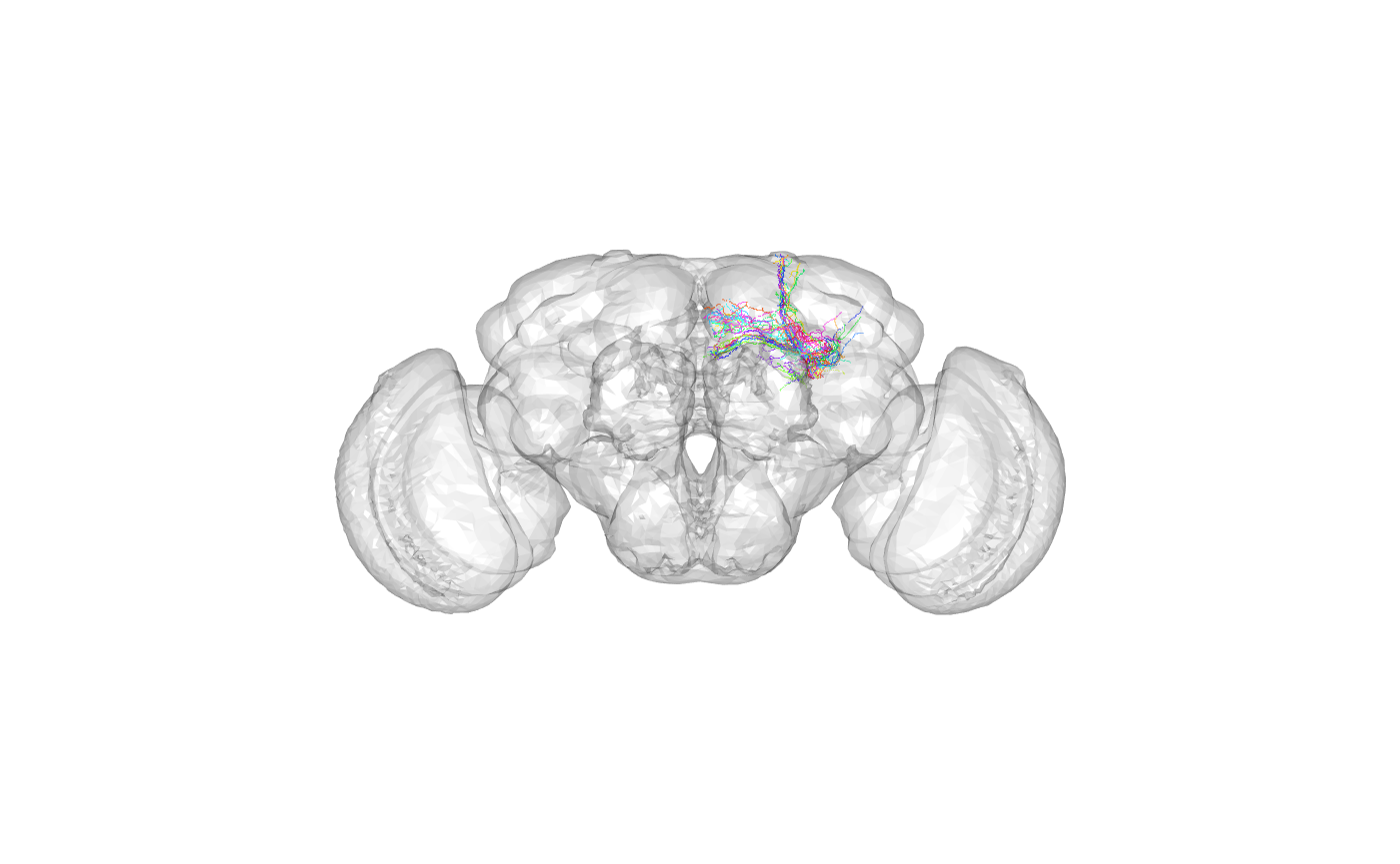
We’ll be plotting these Kenyon cells a lot, so let’s set an option that will save us some typing:
Inspect Kenyon cell NBLAST scores
The package comes with some sample NBLAST scores for a set of 20 Kenyon cells. Each score is a pairwise comparison between two neurons. The score is asymmetric i.e. S(A,B)!=S(B,A). See ?kcs20scores for details.
The scores were computed as follows:
Show the scores for the first five neurons:
##                         FruMARCM-M001205_seg002 GadMARCM-F000122_seg001
## FruMARCM-M001205_seg002               3234.5412                36.80441
## GadMARCM-F000122_seg001                743.0257              3382.60124
## GadMARCM-F000050_seg001                125.6899               244.92594
## GadMARCM-F000142_seg002               1132.1102               212.54249
## FruMARCM-F000270_seg001                214.2611               261.42773
##                         GadMARCM-F000050_seg001 GadMARCM-F000142_seg002
## FruMARCM-M001205_seg002               -935.3377               -251.4999
## GadMARCM-F000122_seg001               -515.5338               -262.2352
## GadMARCM-F000050_seg001               4259.5719                480.4146
## GadMARCM-F000142_seg002                309.9265               4043.1766
## FruMARCM-F000270_seg001               1962.1274                254.7516
##                         FruMARCM-F000270_seg001
## FruMARCM-M001205_seg002               -460.0096
## GadMARCM-F000122_seg001               -145.2588
## GadMARCM-F000050_seg001               2048.0176
## GadMARCM-F000142_seg002                334.3803
## FruMARCM-F000270_seg001               4202.6258
Plotting NBLAST hits
Let’s plot the two neurons that NBLAST thinks are most similar.
Find the indices of the maximum off-diagonal score in the score matrix:
# find the maximum off-diagonal (i.e. non-self match)
max_realmatch=max(kcs20scores[upper.tri(kcs20scores,diag=F)])
ind<-which(kcs20scores==max_realmatch,arr.ind=T)
queryneuron <- colnames(kcs20scores)[ind[2]]
targetneuron <- rownames(kcs20scores)[ind[1]]
What was the query?
## [1] "FruMARCM-F001494_seg002"What was the target?
## [1] "FruMARCM-M001051_seg002"What do they look like and where in the brain are they?
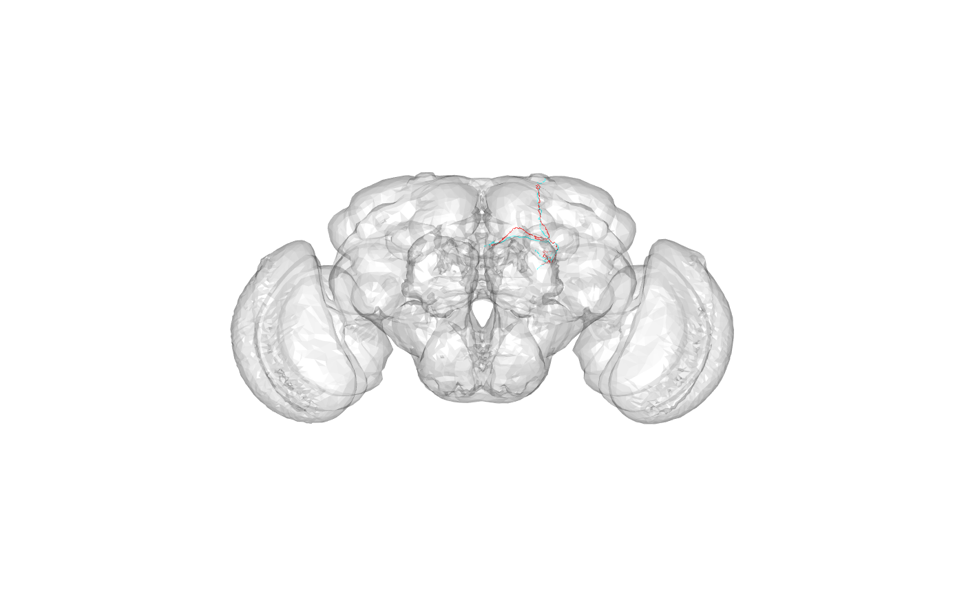 Look like a pair of alpha/beta core Kenyon cells.
Cluster Kenyon cells by morphology
# nb this works because options(flycircuit.scoremat="kcs20scores")
# can also set the score matrix to use explicitly
# hckc <- hclustfc(rownames(kcs20scores), scoremat=kcs20scores)
hckc <- hclustfc(rownames(kcs20scores))
## The "ward" method has been renamed to "ward.D"; note new "ward.D2"library(dendroextras)
par(mar=c(12, 4, 2, 2)) # Extra margin for labels
plot(colour_clusters(hckc, k=3))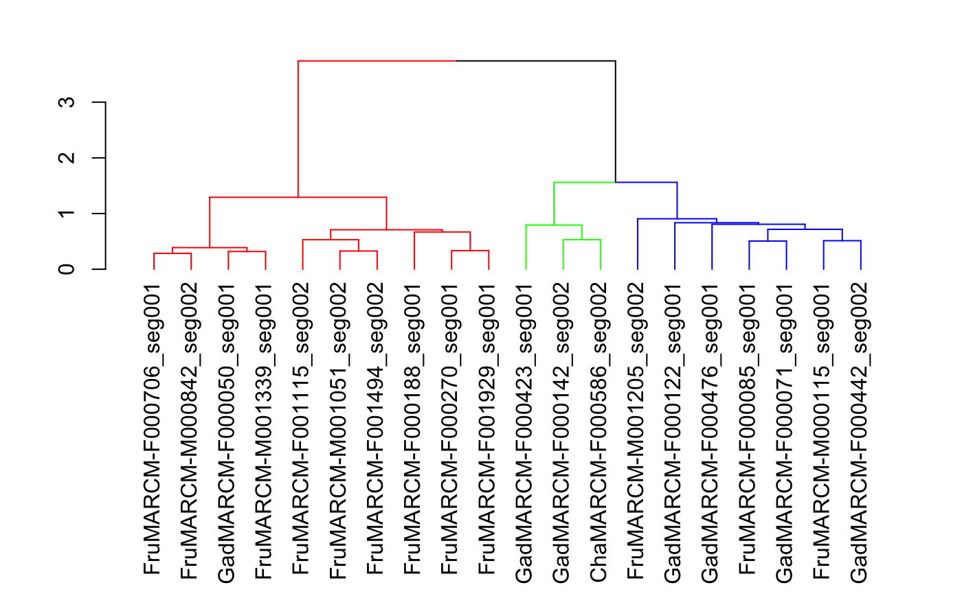
Now let’s look at the neurons:
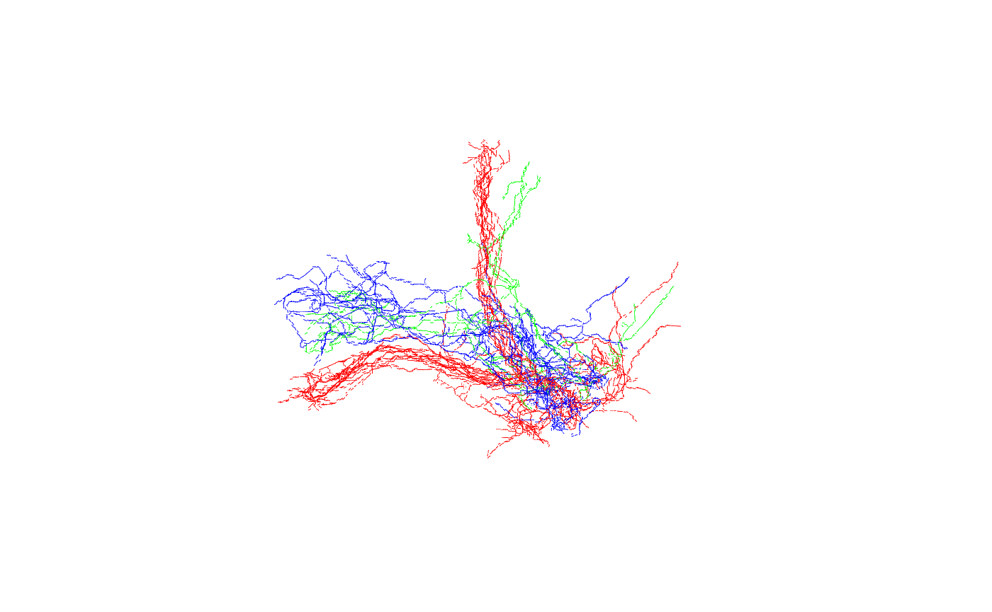 Good, we can see the 3 main classes (gamma, alpha’/beta’ and alpha/beta).
More NBLASTing
We know that FruMARCM-F001494_seg002 and FruMARCM-M001051_seg002 are the two most similar neurons in our subset of 20 Kenyon cells, but how do other neurons compare with FruMARCM-F001494_seg002? Let’s NBLAST it against all the other neurons and look at the scores.
results <- fc_nblast(queryneuron, names(kcs20), 'kcs20scores')
par(las=2) # Horizontal labels
par(mar=c(5, 14, 2, 2)) # Extra margin for labels
barplot(results, horiz=T)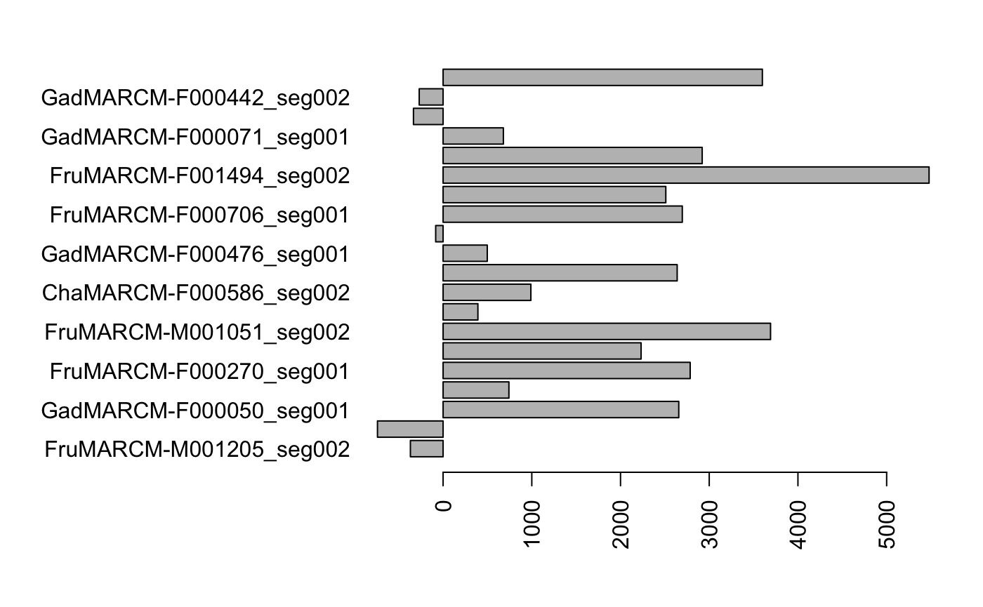 Unsurprisingly, FruMARCM-F001494_seg002 itself has the highest score (seeing as it is exactly the same as itself). Interestingly, while FruMARCM-M001051_seg002 has the second-highest score, FruMARCM-F001929_seg001 has a similarly high score, closely followed by FruMARCM-F000188_seg001 and FruMARCM-F000270_seg001. Let’s plot them all, with the query neuron in black, to see how similar they are:
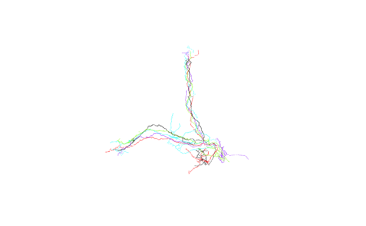 Hmm, they look pretty similar. Let’s plot the four worst hits for comparison:
 Definitely different.