Front-leg sensorimotor loops • bancr

A central claim of the BANC paper (Bates et al. 2026, Nature) is that motor control in Drosophila is distributed — many behaviours are not orchestrated by a single brain command followed by passive execution in the ventral nerve cord (VNC), but instead emerge from local sensorimotor loops embedded inside individual VNC neuromeres, coordinated by ascending and descending pathways.

The front-leg neuromere (T1) is a convenient place to see one of those loops by eye: the leg’s mechanosensory afferents enter through the front-leg nerve, the motor neurons that drive the leg muscles exit through the same nerve, and a population of small VNC intrinsic neurons (the “single-leg-neuromere” cell class) sits between them. In this article we use bancr to identify those intrinsic neurons by the purely connectomic criterion of being monosynaptic between left front-leg sensory neurons and left front-leg motor neurons, then build a public Neuroglancer scene that shows the three groups colour-coded.

Everything below runs against public BANC resources: annotations come from the public GCS snapshot (no authentication required), and synaptic connectivity comes from the read-only public CAVE datastack brain_and_nerve_cord_public.

Setup

Even though every step below runs against public BANC resources, CAVE still requires a personal token tied to your Google account before any of its endpoints will answer. If you haven’t set one up yet, run banc_set_token() once — it opens a browser, signs you in via Google, and stashes the token for future sessions. The bancr README walks through the full setup. No production-access grant is needed to follow this article; the token alone is enough.

library(bancr)
library(dplyr)

# Pin every CAVE call in this article to the public read-only
# datastack so the analysis works without production access.
options(bancr.datastack = "brain_and_nerve_cord_public")

Load the codex annotation table

banc_codex_annotations() returns a per-neuron pivot of the BANC codex annotation table — the same one displayed at https://codex.flywire.ai/?dataset=banc. By default it reads from a cached public GCS snapshot, so this first call needs no CAVE token.

codex <- banc_codex_annotations()

Select left-front-leg sensory and motor pools

The codex carries the BANC annotation hierarchy (super_class, cell_class, cell_sub_class, cell_type) plus laterality (side), the sensed body part (body_part_sensory) and the motor target (body_part_effector). We filter to neurons whose receptive or motor field is the left front leg.

sensory <- codex %>%
  filter(
    super_class == "sensory",
    side == "left",
    grepl("front_leg", body_part_sensory)
  )

motor <- codex %>%
  filter(
    grepl("motor", super_class),
    side == "left",
    grepl("front_leg", body_part_effector)
  )

c(sensory = nrow(sensory), motor = nrow(motor))
#> sensory   motor 
#>     836      69

Find intrinsic neurons that close the loop

To be on the loop, an intrinsic neuron must receive direct input from at least one of the sensory neurons and send direct output to at least one of the motor neurons. We use banc_partner_summary() to pull the monosynaptic partner lists, one row per (query neuron → partner) edge.

version = 888 pins the call to the most recent materialisation exposed by the public datastack. We deliberately pass threshold = 0 so the partners step keeps every candidate edge; the cell-class and side filters below do the tightening.

sensory_out <- banc_partner_summary(
  sensory$pt_root_id,
  partners = "outputs",
  threshold = 0,
  version = 888
)

motor_in <- banc_partner_summary(
  motor$pt_root_id,
  partners = "inputs",
  threshold = 0,
  version = 888
)

candidates <- intersect(
  as.character(sensory_out$post_id),
  as.character(motor_in$pre_id)
)
length(candidates)
#> [1] 2229

The intersection of “downstream of any sensory neuron” and “upstream of any motor neuron” is still loose — it includes brain interneurons, contralateral pathways and projection neurons that just happen to touch both ends. We tighten to a clean local-circuit population by restricting to the single_leg_neuromere cell class on the same (left) side.

intrinsic <- codex %>%
  filter(
    as.character(pt_root_id) %in% candidates,
    cell_class == "single_leg_neuromere",
    side == "left"
  )

nrow(intrinsic)
#> [1] 255

A quick breakdown by cell_sub_class gives a sense of the sub-populations involved:

intrinsic %>%
  count(cell_sub_class, sort = TRUE) %>%
  head(10)
#> # A tibble: 4 × 2
#>   cell_sub_class                                     n
#>   <chr>                                          <int>
#> 1 ventral_nerve_cord_ipsilateral_restricted        231
#> 2 ventral_nerve_cord_bilateral_restricted           15
#> 3 ventral_nerve_cord_bilateral_interconnecting       6
#> 4 ventral_nerve_cord_ipsilateral_interconnecting     3

Render a sample of the loop in BANC space

Before we build the full interactive scene, here’s a quick static look at the geometry. We sample a handful of neurons per group, pull their meshes from the public BANC bucket, decapitate them at the neck connective to keep only the VNC portion, and lay out a 3 × 2 grid: one column per group (sensory, intrinsic, motor), one row per view (VNC dorsal, VNC lateral). Each group has its own colour ramp (blues / greens / reds) with within-group jitter so individual neurons remain visually separable.

library(ggplot2)
library(patchwork)

set.seed(1)
sample_ids <- list(
  sensory   = sample(sensory$pt_root_id,   4),
  intrinsic = sample(intrinsic$pt_root_id, 4),
  motor     = sample(motor$pt_root_id,     4)
)

sens_m <- banc_read_neuron_meshes(sample_ids$sensory)
#> Warning: deduplication not currently supported for this layer's variable layered draco meshes
#> Warning: deduplication not currently supported for this layer's variable layered draco meshes
#> Warning: deduplication not currently supported for this layer's variable layered draco meshes
#> Warning: deduplication not currently supported for this layer's variable layered draco meshes
intr_m <- banc_read_neuron_meshes(sample_ids$intrinsic)
#> Warning: deduplication not currently supported for this layer's variable layered draco meshes
#> Warning: deduplication not currently supported for this layer's variable layered draco meshes
#> Warning: deduplication not currently supported for this layer's variable layered draco meshes
#> Warning: deduplication not currently supported for this layer's variable layered draco meshes
mot_m  <- banc_read_neuron_meshes(sample_ids$motor)
#> Warning: deduplication not currently supported for this layer's variable layered draco meshes
#> Warning: deduplication not currently supported for this layer's variable layered draco meshes
#> Warning: deduplication not currently supported for this layer's variable layered draco meshes
#> Warning: deduplication not currently supported for this layer's variable layered draco meshes

# Per-group colour ramps (same families banc_neuron_comparison_plot
# uses, expanded across the N neurons per group so they stay
# visually distinct).
pal_sensory   <- grDevices::colorRampPalette(
  c("#00008B","#0000CD","#4169E1","#1E90FF","#87CEEB","#B0E0E6"))
pal_intrinsic <- grDevices::colorRampPalette(
  c("#006400","#076b3e","#228B22","#32c080","#90EE90"))
pal_motor     <- grDevices::colorRampPalette(
  c("#8f0723","#DC143C","#FF4500","#FF7F50","#F88379","#FFB6C1"))

make_panel <- function(neurons, view, palette, label, label_colour) {
  rotation <- banc_rotation_matrices[[view]]
  ggplot() +
    nat.ggplot::geom_neuron(
      x = bancr::banc_vnc_neuropil.surf,
      rotation_matrix = rotation,
      alpha = 0.05, cols = c("grey90", "grey60")
    ) +
    nat.ggplot::geom_neuron(
      x = banc_decapitate(neurons, invert = FALSE),
      rotation_matrix = rotation,
      cols = palette(length(neurons)),
      alpha = 0.85, linewidth = 0.3
    ) +
    coord_fixed() +
    theme_void() +
    ggtitle(label) +
    theme(
      plot.title = element_text(hjust = 0, size = 9,
                                face = "bold", colour = label_colour),
      legend.position = "none"
    )
}

groups <- list(
  sensory   = list(neurons = sens_m, palette = pal_sensory,   colour = "#1E90FF"),
  intrinsic = list(neurons = intr_m, palette = pal_intrinsic, colour = "#228B22"),
  motor     = list(neurons = mot_m,  palette = pal_motor,     colour = "#DC143C")
)

views <- c(dorsal = "vnc", lateral = "vnc_side")

panels <- list()
for (v in names(views)) {
  for (g in names(groups)) {
    panels[[paste(v, g, sep = "_")]] <- make_panel(
      groups[[g]]$neurons,
      views[[v]],
      groups[[g]]$palette,
      sprintf("%s — %s", g, v),
      groups[[g]]$colour
    )
  }
}

patchwork::wrap_plots(panels, ncol = 3)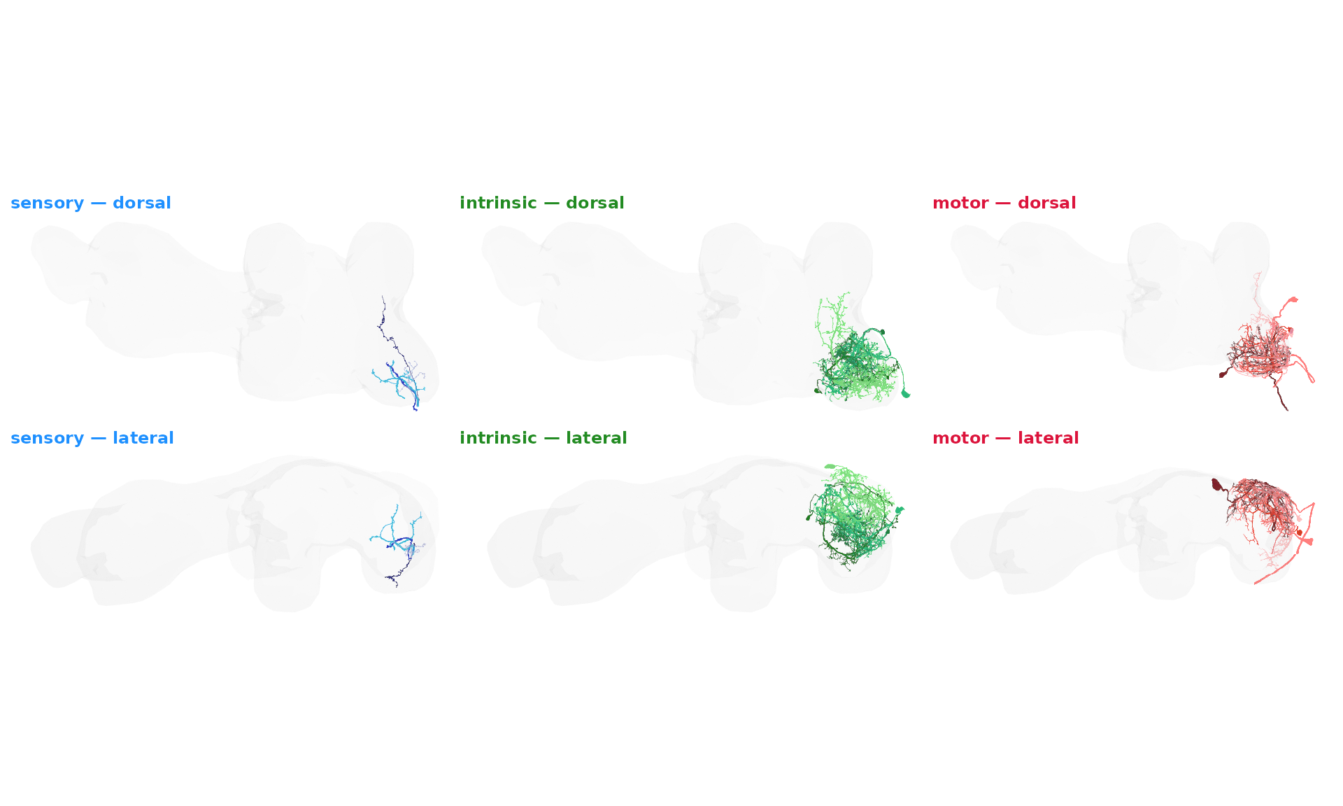

Sample left-front-leg sensory, intrinsic and motor neurons in the VNC, each group in its own colour ramp, shown in dorsal and lateral views

The motor and intrinsic arbours hug the left T1 neuromere, and the sensory afferents enter through the front-leg nerve and ramify in the same volume — exactly the local-loop geometry the BANC paper emphasises.

Render the loop as a public Neuroglancer scene

banc_scene() returns the canonical public BANC Neuroglancer state. We decode it, set the segmentation-proofreading layer’s segment list to the union of our three pools, colour each id by its super_class, and shorten the resulting URL via banc_shorturl().

# Group → colour map (colour-blind-safe Okabe-Ito palette)
group_colours <- c(
  sensory   = "#0072B2",  # blue
  intrinsic = "#009E73",  # green
  motor     = "#D55E00"   # vermillion
)

# One row per neuron with its id and group colour
colourdf <- bind_rows(
  data.frame(ids = as.character(sensory$pt_root_id),
             col = group_colours[["sensory"]]),
  data.frame(ids = as.character(intrinsic$pt_root_id),
             col = group_colours[["intrinsic"]]),
  data.frame(ids = as.character(motor$pt_root_id),
             col = group_colours[["motor"]])
)

# Build the scene: load the base public BANC state, install the
# segment list on the proofreading layer, then layer the colour map
# on top. The base scene archives the proofreading layer and selects
# "BANC static" by default — flip both so the reader opens the link
# straight onto our coloured neurons.
sc <- fafbseg::ngl_decode_scene(banc_scene())
layer_idx <- match("segmentation proofreading",
                   sapply(sc$layers, `[[`, "name"))
sc$layers[[layer_idx]]$segments <- colourdf$ids
sc$layers[[layer_idx]]$archived <- FALSE
sc$selectedLayer <- list(visible = TRUE,
                         layer = "segmentation proofreading")

scene_url <- fafbseg::ngl_add_colours(
  as.character(sc),
  colourdf,
  layer = "segmentation proofreading"
)

short_url <- banc_shorturl(scene_url)
short_url
#> [1] "https://spelunker.cave-explorer.org/#!middleauth+https://global.daf-apis.com/nglstate/api/v1/6393410721153024"

Open the front-leg sensorimotor scene in Spelunker

The Neuroglancer scene shows the 836 sensory neurons in blue, the 255 single-leg-neuromere intrinsic neurons in green, and the 69 motor neurons in vermillion. Switching on a neuropil overlay makes it obvious that the whole loop sits inside the T1 left neuromere — exactly the local sensorimotor module the BANC paper highlights.

Exporting the loop for downstream analysis

A common follow-up is to share the full list of root IDs and their annotations with collaborators (e.g. for proofreading, for matching against another connectome, or for use in a non-R workflow). The analysis output is a single tidy data frame — bind the three pools, keep the annotation columns you care about, and write to CSV.

loop_selection <- dplyr::bind_rows(
  sensory   |> dplyr::mutate(group = "sensory"),
  intrinsic |> dplyr::mutate(group = "intrinsic"),
  motor     |> dplyr::mutate(group = "motor")
) |>
  dplyr::select(
    group, pt_root_id,
    super_class, cell_class, cell_sub_class, cell_type,
    side, body_part_sensory, body_part_effector,
    nerve, hemilineage
  )

write.csv(loop_selection,
          file = "~/Downloads/front_leg_sensorimotor_loop.csv",
          row.names = FALSE)

What next

This is a single, manually-defined slice of the distributed-control architecture characterised in Bates et al. 2025. The same recipe — a codex filter for the two endpoints, a partners-API intersection, a cell-class filter for the intrinsic pool — extends naturally to other body parts (body_part_sensory / body_part_effector), other sides, and other intrinsic cell classes (sequential_leg_neuromeres, intrasegmental, …). For whole-CNS analyses, swap the per-query banc_partner_summary() calls for the precomputed banc_edgelist() / banc_edgelist_split() snapshots (also public, also GCS-backed) and join against the codex table in dplyr.