FAFB-FlyWire • fafbseg

Introduction

This articles gives a quick overview of mapping points between FAFB14 (as used by the “walled garden” and Virtual Fly Brain and FlyWire.

library(fafbseg)
#> Run dr_fafbseg() for a status report on your installation

Basic point mapping

Some known points

# identified location in FAFB14
p.fafb.nm <- cbind(477042, 284535, 90680)
p.fafb.raw <- p.fafb.nm/c(4,4,40)
# corresponding location in FlyWire
p.flywire.raw <- cbind(118865, 71338, 2267)
p.flywire.nm <- p.flywire.raw * c(4,4,40)

Compare displacements (in nm) for forward or inverse mapping

# check displacement
flywire2fafb(p.flywire.nm)-p.fafb.nm
#>      X  Y Z
#> [1,] 3 -1 0

# check what happens when you apply the inverse
fafb2flywire(p.fafb.nm)-p.flywire.nm
#>       X Y Z
#> [1,] -3 2 0

A sample neuron. First map the points

data("AV4b1", package='catmaid')
before=xyzmatrix(AV4b1)
after=fafb2flywire(before)

Then some stats and a quick histogram

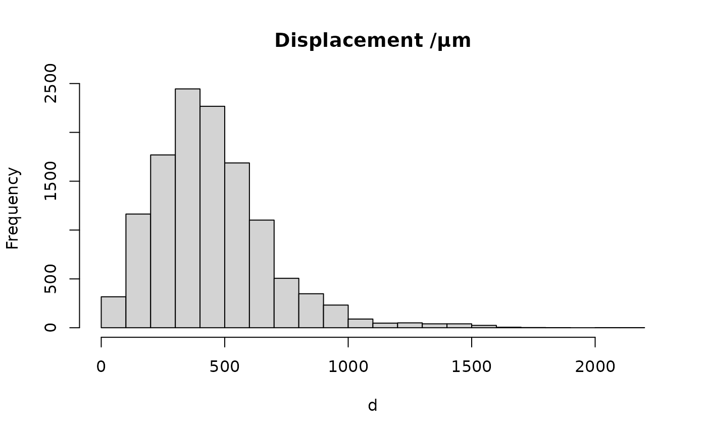
d=sqrt(rowSums((before-after)^2))
summary(d)
#>    Min. 1st Qu.  Median    Mean 3rd Qu.    Max. 
#>     2.0   287.9   416.0   446.9   559.1  2113.7

hist(d, br=20, main='Displacement /µm')

sample_points_in_surf <- function(x, n){
  x=as.mesh3d(x)
  bb=boundingbox(x)
  mm=mapply(runif, min=bb[1,], max=bb[2,], n = n)
  colnames(mm)=c("X","Y","Z")
  data.frame(mm, inside=pointsinside(mm,x))
}

set.seed(42)
sxyz=sample_points_in_surf(FAFB14.surf,25000)
sxyz.in=subset(sxyz, inside)
sxyz.fw=fafb2flywire(xyzmatrix(sxyz.in))
deltas=sxyz.fw-sxyz.in
delta=rowSums(deltas[,c("X","Y")])

jet.colors<-colorRampPalette(c('navy','cyan','yellow','red'))
nclear3d();
spheres3d(xyzmatrix(sxyz.in), col=jet.colors(10)[cut(delta, breaks = 10)], rad=2000)

Round trip error

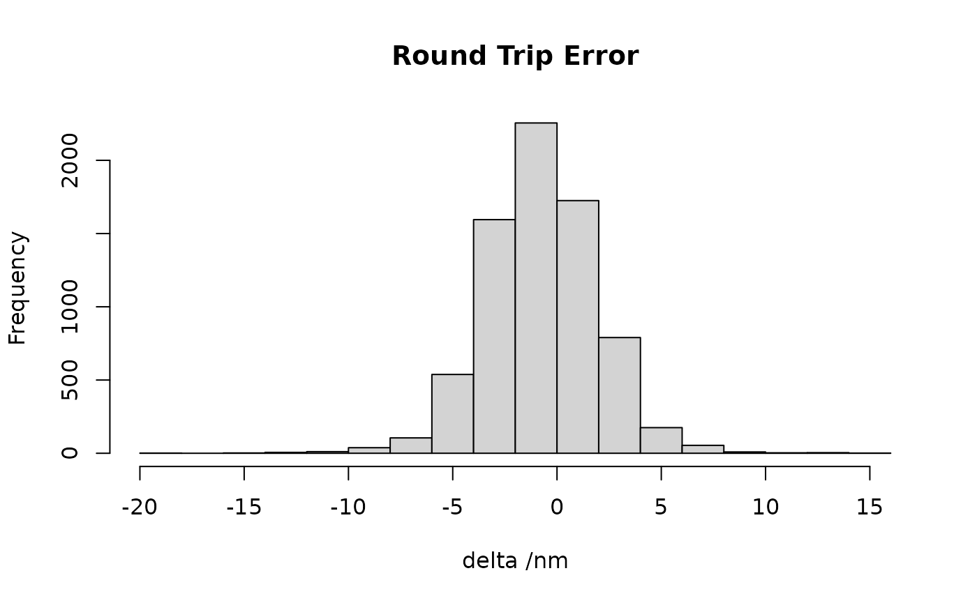
Let’s send those points back again

sxyz.fafb2=flywire2fafb(sxyz.fw)

deltas=sxyz.fafb2-xyzmatrix(sxyz.in)
delta=rowSums(deltas[,c("X","Y")])
hist(delta, main = "Round Trip Error", xlab='delta /nm')

Mapping anything

To map complex objects, use xform_brain()

AV4b1.fw=xform_brain(AV4b1, sample='FAFB14', reference = 'FlyWire')

# find the main branch point of a neuron, a good place to point to
mainbranch <- function(x, ...) {
  if(is.neuronlist(x)) 
    return(nlapply(x, mainbranch, ...))
  
  sx=nat::simplify_neuron(x, ...)
  xyzmatrix(sx)[sx$BranchPoints,]
}

choose_segmentation("flywire")
open_fafb_ngl(mainbranch(AV4b1.fw), coords.only = TRUE)
#> [1] "88371.25,40478.75,3668"

catmaid catmaid

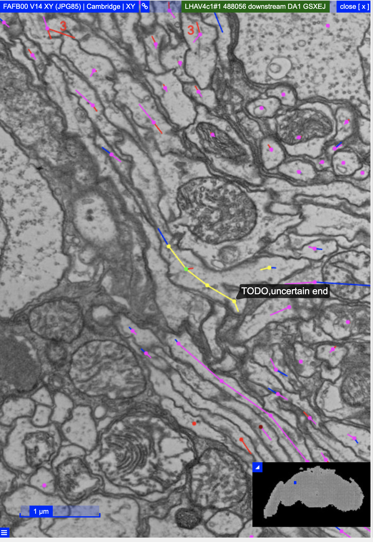
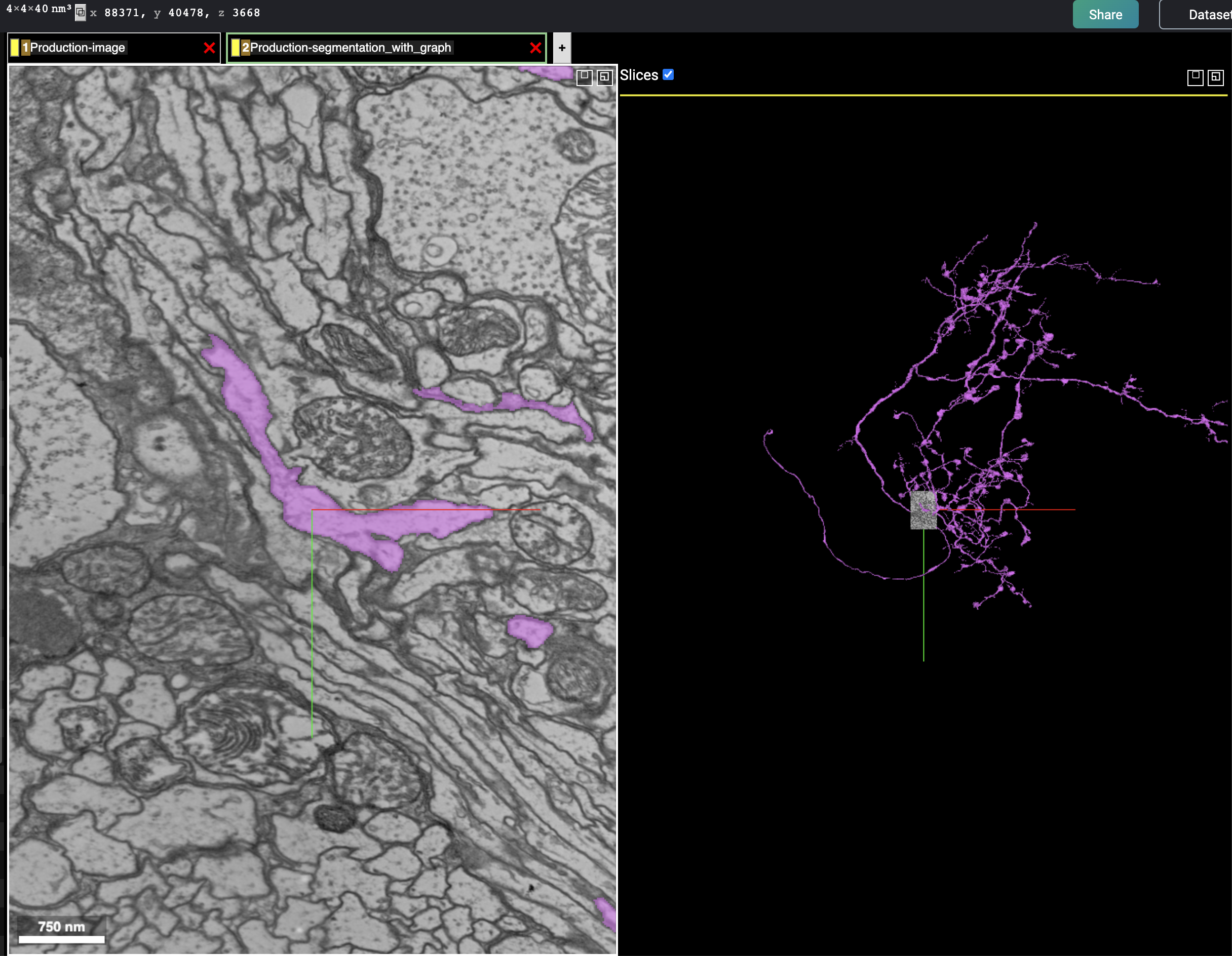
Note the relevant links:

Load the flywire mesh

av4.fwm=read_cloudvolume_meshes('720575940618054533')

And plot with the CATMAID skeleton

nclear3d()
plot3d(AV4b1.fw, col='red', lwd=3)

wire3d(av4.fwm[[1]], col='grey', alpha=.2)