NeuroGeometry: Analysing 3D morphology of neurons
Gregory Jefferis
2022-01-09
Source:vignettes/NeuroGeometry.Rmd
NeuroGeometry.RmdIntroduction
One of the key distinguishing features of nat is the ability to analyse neuronal morphology and connectivity from a geometric perspective. In other words nat provides functions to analyse the placement of neurons within the context of the brain and the organisation of local circuits.
This vignette will give a few examples, but this is only skimming the surface of what is possible.
If you see an analysis in a paper associated with the Jefferis lab but cannot figure out how to use nat to achieve this, then feel free to contact the nat–user Google group to ask for help.
Vertex information
## Loading required package: rgl## Registered S3 method overwritten by 'nat':
## method from
## as.mesh3d.ashape3d rgl##
## Attaching package: 'nat'## The following object is masked from 'package:rgl':
##
## wire3d## The following objects are masked from 'package:base':
##
## intersect, setdiff, unionOne of the key tools for geometric work in nat is the xyzmatrix function, which extracts 3-D coordinate information from any object containing vertices.
##        X               Y                Z
##  Min.   :186.9   Min.   : 90.36   Min.   : 88.2
##  1st Qu.:225.6   1st Qu.: 97.56   1st Qu.:103.4
##  Median :258.4   Median :102.70   Median :112.9
##  Mean   :249.4   Mean   :104.03   Mean   :120.9
##  3rd Qu.:277.7   3rd Qu.:109.04   3rd Qu.:139.0
##  Max.   :289.5   Max.   :132.71   Max.   :157.3
This also works for neuronlists, so we can extract all of the points in a collection of neurons:
xyz=xyzmatrix(Cell07PNs)We could ask for all the points close to a specific X coordinate
## close_to_x250
## FALSE  TRUE
## 20479  1728
We can also select points interactively by using the rgl::select3d function.
Worked example - plane cutting a tract
As a worked example let’s try to find the plane cutting a tract defined by the axons of some example neurons:
plot(Cell07PNs, WithNodes=F)
dist=10
abline(v=250, col='red')
abline(v=c(250-dist, 250+dist), col='red', lty='dotted')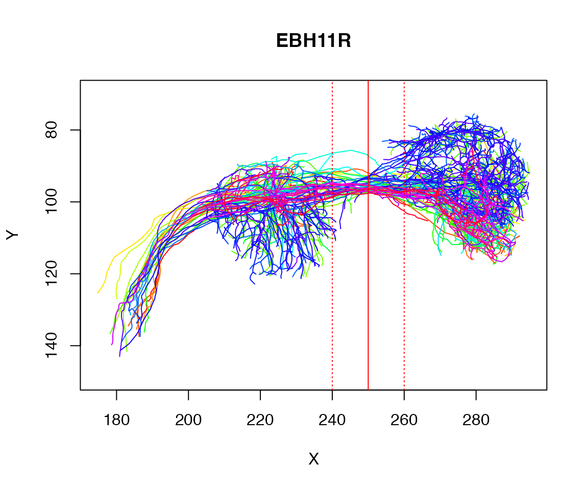
We could ask for all the points close to a specific X coordinate
## close_to_x250
## FALSE  TRUE
## 20479  1728
Let’s find the centroid of those selected points:
centroid=colMeans(xyz[close_to_x250,])
centroid
## X Y Z
## 251.16788 94.76735 141.11495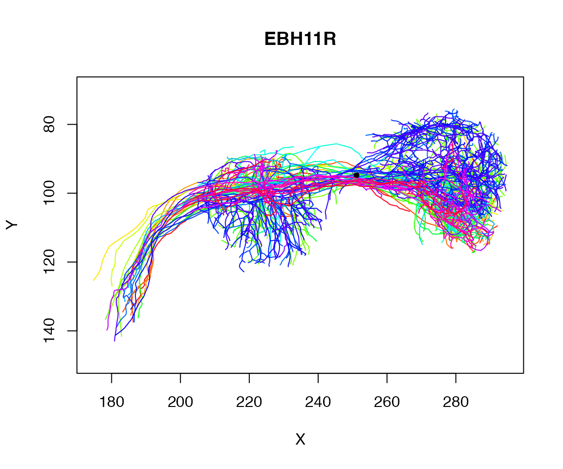
PCA to find tract vector
Now let’s do a principal components analysis on those points
pc=prcomp(xyz[close_to_x250,])
pc1=pc$rotation[,'PC1']
plot(Cell07PNs, WithNodes=F)
points(matrix(centroid[1:2],ncol=2), pch=20)
res=rbind(centroid-pc1*10, centroid, centroid+pc1*10)
lines(res[,1:2])
OK, perhaps it would be better if we only used the spine of the neurons
# There is a problem with one neuron with a loop, hence OmitFailures
spines=nlapply(Cell07PNs, spine, UseStartPoint=T, OmitFailures = T)
## Warning in get.shortest.paths(ng, from = from, to = to, mode = "all"): At
## structural_properties.c:4745 :Couldn't reach some vertices## close_to_x250
## FALSE TRUE
## 5137 876
pc=prcomp(xyz[close_to_x250,])
pc1=pc$rotation[,'PC1']
plot(spines, WithNodes=F)
points(matrix(centroid[1:2],ncol=2), pch=20)
res=rbind(centroid-pc1*10, centroid, centroid+pc1*10)
# nb 1:2 => just the xy coords
lines(res[,1:2])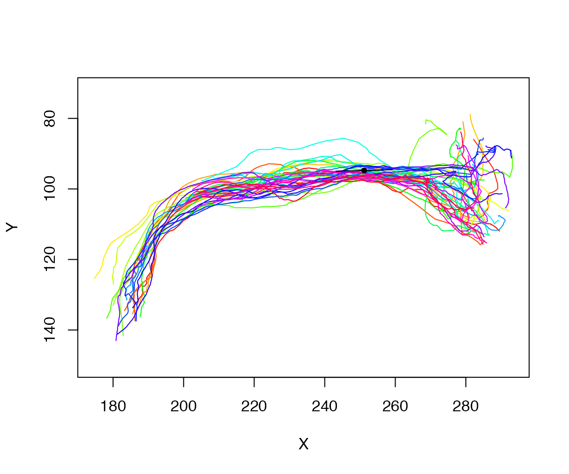
Tract vector for each neuron
Alternatively, we could find the vector of the first PC for each neuron. Let’s write a function to do that and then apply it to the spine of each neuron.
# returns 6 vector
# first 3 values are centroid
# second three values first principal component
tract_vector <- function(n, xval=250, thresh=10) {
  p=xyzmatrix(n)
  near=abs(p[,'X']-xval)<thresh
  pc=prcomp(p[near,])
  c(colMeans(p[near,]), pc$rotation[,'PC1'])
}
tvs=sapply(spines, tract_vector)
mean_cent=rowMeans(tvs[1:3,])
mean_vec=rowMeans(tvs[4:6,])

# nb *10 to make the vector longer (10 µm) and more visible
res2=rbind(mean_cent-mean_vec*10, mean_cent, mean_cent+mean_vec*10)
plot(spines, col='grey', WithNodes=F)
lines(res2[,1:2], lwd=3)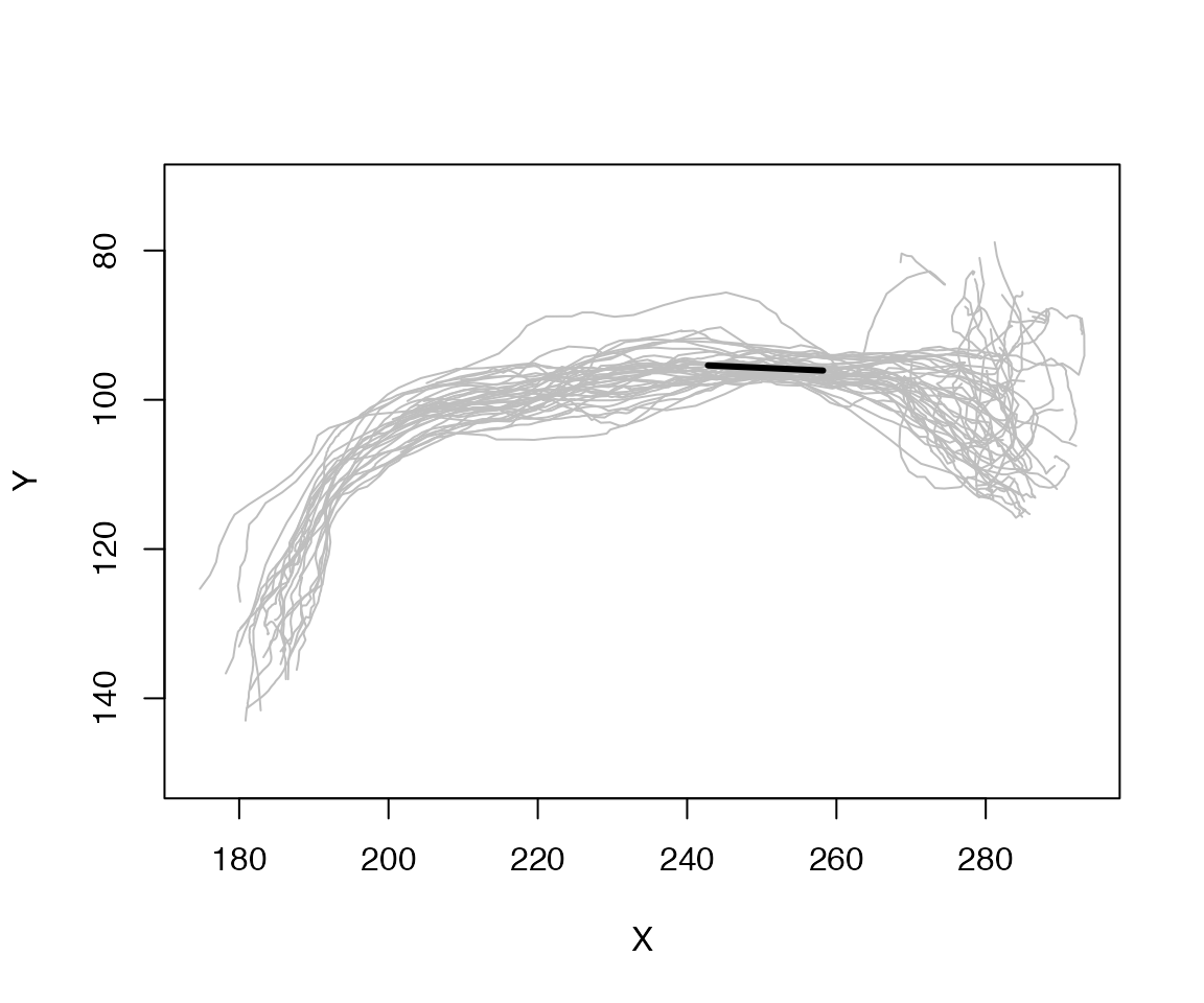
Lines crossing a plane
We can look at the plane we have defined in a 3D context as follows:
plc=plane_coefficients(mean_cent, mean_vec)
plot3d(Cell07PNs[c(1,30)], col='grey', WithNodes = F)
planes3d(plc[,1:3], d=plc[,'d'])
We can also make a small square plane centred on the chosen point
library(rgl)
clear3d()
make_centred_plane <- function(point, normal, scale = 1) {
  # find the two orthogonal vectors to this one
  uv = Morpho::tangentPlane(normal)
  uv = sapply(uv, "*", scale, simplify = F)
  qmesh3d(
  cbind(
  point + uv$z,
  point + uv$y,
  point - uv$z,
  point - uv$y
  ),
  homogeneous = F,
  indices = 1:4
  )
}
plane=make_centred_plane(mean_cent, mean_vec, scale=15)
plot3d(spines, col='grey')
shade3d(plane, col='red')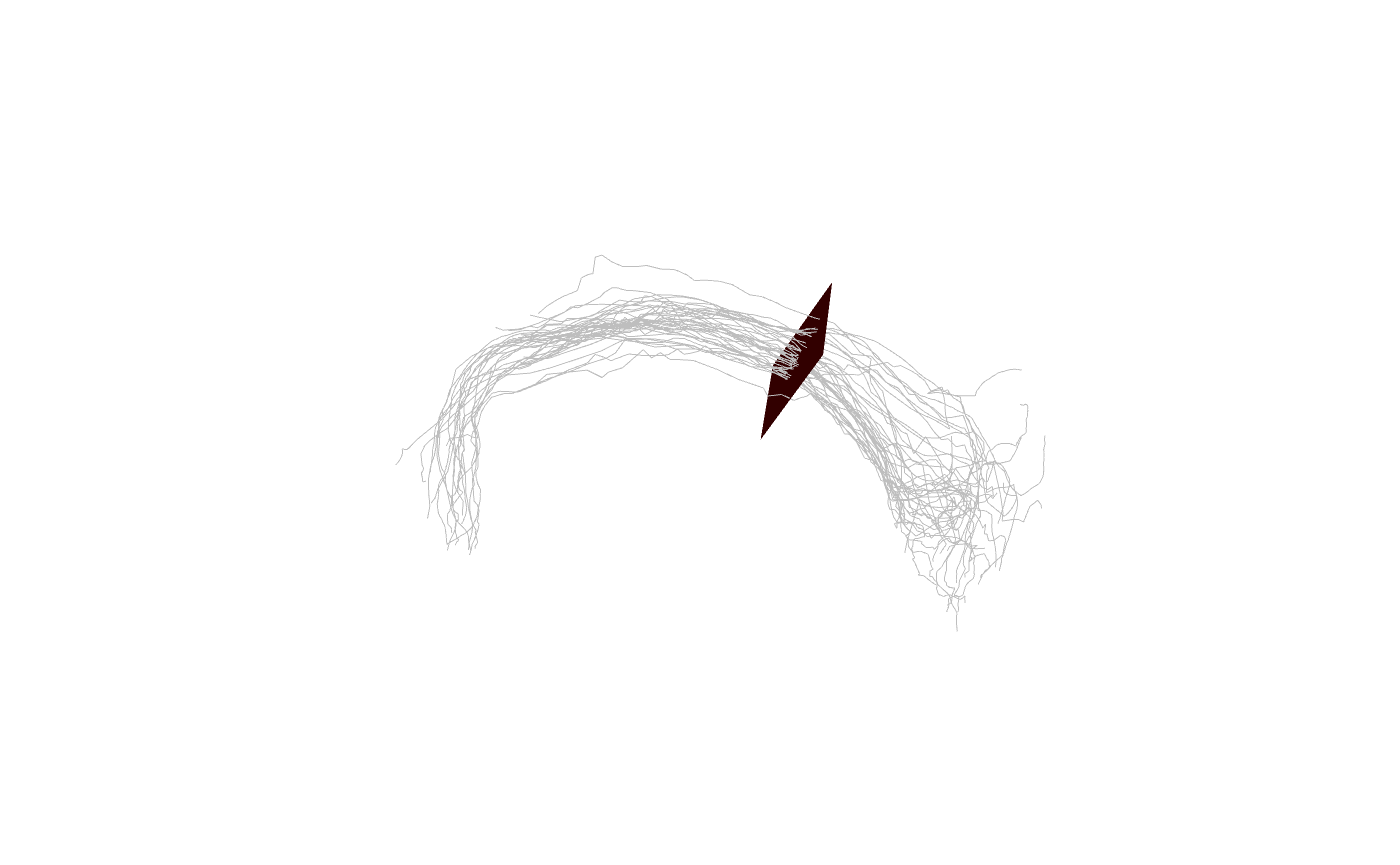
Finally, we can find the positions at which each neuron intersects the plane. Note that when there are multiple intersections, we only choose the closest point to the centroid that we calculated when defining the plane.
intersections=t(sapply(Cell07PNs, intersect_plane, plc, closestpoint=mean_cent))
# center those intersection points
intersections.cent=scale(intersections, center = T, scale = F)
d=sqrt(rowSums(intersections.cent^2))
mean(d)
## [1] 3.118692Then we can plot those positions on the plane
Finally we can construct a 2D coordinate system on the plane and project the intersection positions onto that.
# find pair of orthogonal tangent vectors of plane
uv = Morpho::tangentPlane(mean_vec)
# centre our points on mean
sp=scale(intersections, scale = F, center=T)
DotProduct=function(a,b) sum(a*b)
# find coordinates w.r.t. to our two basis vectors
xy=data.frame(u=apply(sp, 1, DotProduct, uv[[1]]),
           v=apply(sp, 1, DotProduct, uv[[2]]))
# maintain consist x-y aspect ratio
plot(xy, pch=19, asp=1, main = "Position of Axon intersection in plane",
     xlab="u /µm", ylab="v /µm")