Finding the SEZ AstA neuron: SS32423 + AstA-locus drivers + DCV soma scores
Source:vignettes/asta_sez.Rmd
asta_sez.RmdOverview
The split-GAL4 line SS32423 (Sterne et al. 2021, the
aMulet line) is reported to label an Allatostatin-A
(AstA)-expressing neuron of the subesophageal zone (SEZ), but
only weakly. Both of its hemidrivers sit in the AstA locus on 3R — the
AD half is VT019900 and the DBD half is R65D06
— and the canonical “AstA-GAL4” Pfeiffer tile R65D05
(Hergarden et al. 2012) is the immediate neighbour of
R65D06 on the chromosome. Together with R65D07
and a few flanking tiles these enhancers form a natural panel of
AstA-locus drivers, and any FlyWire-FAFB-v783 neuron
they all match should be a strong candidate for “the” SEZ AstA cell.
This vignette chains four resources to converge on a small ranked candidate list of FAFB-v783 neurons that:
- match SS32423 and its sibling AstA-locus drivers in NeuronBridge
colour-depth search (release
v3_9_0); - have a soma in an SEZ neuropil (GNG, SAD, AMMC, FLA);
- score in the top ~10th percentile of central-brain
soma_dcv_density— the dense-core-vesicle proxy for being peptidergic — consistent with secreting AstA; - visually agree with the SS32423 NeuronBridge MIP.
The output is a small ranked list, and a comparison figure showing the SS32423 NeuronBridge MIP next to the candidate FlyWire neuron(s) you would take into experiments.
A reproducer for everything below lives at
inst/scripts/run_asta_sez.R — running it regenerates the
figures in inst/images/ and the ranked CSVs in
inst/extdata/asta_sez/.
Prerequisites
if (!require("remotes")) install.packages("remotes")
remotes::install_github("natverse/neuronbridger")
remotes::install_github("natverse/fafbseg")
remotes::install_github("natverse/nat.flybrains")
remotes::install_github("natverse/nat.templatebrains")
remotes::install_github("natverse/nat.jrcbrains")
install.packages(c("arrow", "dplyr", "tidyr", "ggplot2", "ggrepel"))
library(neuronbridger)
library(arrow); library(dplyr); library(tidyr); library(ggplot2)

NB_VERSION <- "v3_9_0"   # current release; ships FlyWire-FAFB-v783 MIPs
Local feather caches of the lee-lab compiled FAFB-v783 tables (see
/Users/GD/LMBD/Papers/dcv for the DCV scoring
methodology):
Step 1: Build the AstA-locus driver panel
The panel is built by hand from the literature: SS32423 plus the GMR
and VT enhancer fragments that tile the AstA locus and have FlyLight
imaging in NeuronBridge. R65D04 is included in the
literature but absent from NB v3_9_0 — confirm and drop it on the
fly.
driver_panel <- tibble::tribble(
  ~line,        ~role,
  "SS32423",    "primary lead — aMulet split (Sterne et al. 2021); both halves AstA-locus",
  "R65D05",     "Pfeiffer 'AstA-GAL4' (Hergarden 2012; Pool 2014; Landayan 2021)",
  "R65D06",     "DBD half of SS32423 — Pfeiffer tile in AstA locus",
  "R65D04",     "neighbouring AstA-locus tile — absent from NB v3_9_0",
  "R65D07",     "neighbouring AstA-locus tile",
  "R65E01",     "neighbouring AstA-locus tile",
  "VT019900",   "AD half of SS32423 — Vienna Tile in AstA locus"
)
Confirm and select brain MIPs (FAFB hits only come from brain MIPs,
not VNC ones). NB stores many redundant MIPs per line — broad lines have
50+ — and neuronbridge_hits() calls
plyr::rbind.fill() internally which is quadratic in the
number of result rows, so we cap at 5 MIPs per line. Multiple MIPs of
the same line are slightly different stainings of the same GAL4, and
slice_max() downstream takes the best score per neuron, so
5 is plenty.
panel_info <- list()
for (ln in driver_panel$line) {
  out <- try(neuronbridge_info(ln, dataset = "by_line",
                               version = NB_VERSION), silent = TRUE)
  if (inherits(out, "try-error") || !nrow(out)) next
  brain <- out[out$anatomicalArea == "Brain", , drop = FALSE]
  if (!nrow(brain)) next
  brain <- head(brain, 10)
  brain$line <- ln
  panel_info[[ln]] <- brain
}
panel_info <- bind_rows(panel_info)
# In v3_9_0: SS32423 (16 brain MIPs), R65D05 (75), R65D06 (60), R65D07
# (15), R65E01 (48), VT019900 (21); R65D04 absent. Capped at 10 → 60
# MIPs total.
Step 2: Pull NeuronBridge FAFB-v783 hits per line
SS32423 itself ships 16 brain MIPs (different specimens — useful to inspect). Most show the same SS32423 pattern, but one or two are MCFO-stochastic stains where only a subset of cells happens to be labelled. Always inspect the full set before choosing a “representative” MIP for the side-by-side comparison:
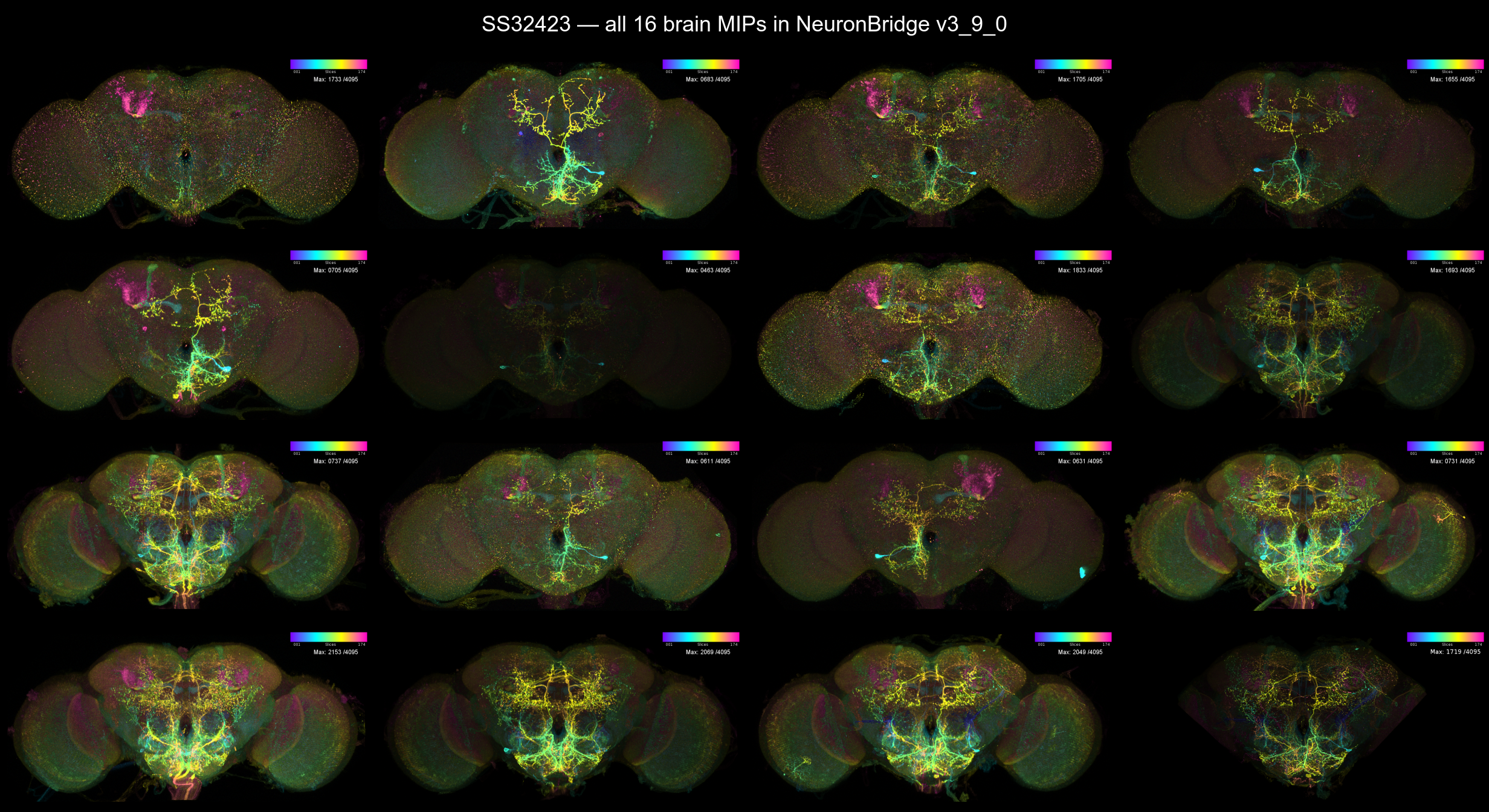
The dominant pattern across the 16 MIPs is a bilateral pair
of cell bodies in the SEZ at the bottom of the brain, with arbours
ascending dorso-medially through the central brain. That’s the
SEZ AstA cell SS32423 was designed to label; the bright single-cell
cluster in the upper-medial brain that appears in only one MIP
(SS32423#3 in this release) is an MCFO stochastic
single-cell render of one of the ascending arbours, not a separate cell
type.
For each driver, fetch its colour-depth hits, restrict to
FlyWire-FAFB (libraryName == "FlyWire_FAFB_v783_realign"),
and cache per line so the slow part doesn’t have to run again.
KEEP_COLS <- c("publishedName","libraryName","normalizedScore",
               "matchingPixels","alignmentSpace","anatomicalArea","gender")
hits_list <- list()
for (ln in unique(panel_info$line)) {
  ln_mips <- panel_info[panel_info$line == ln, ]
  rows <- list()
  for (i in seq_len(nrow(ln_mips))) {
    h <- try(neuronbridge_hits(ln_mips$nb.id[i], version = NB_VERSION),
             silent = TRUE)
    if (inherits(h, "try-error") || is.null(h) || !nrow(h)) next
    h <- h[grepl("FlyWire", h$libraryName), , drop = FALSE]
    if (!nrow(h)) next
    h <- as.data.frame(h[, intersect(KEEP_COLS, colnames(h)), drop = FALSE])
    h$normalizedScore <- as.numeric(h$normalizedScore)
    h$query_line <- ln
    h$query_mip  <- ln_mips$nb.id[i]
    rows[[length(rows)+1L]] <- h
  }
  hits_list[[ln]] <- if (length(rows)) bind_rows(rows) else tibble()
}
hits_raw <- bind_rows(hits_list)
hits_raw$root_783 <- sub("^flywire_fafb:v783:", "", hits_raw$publishedName)
# Live numbers (cap=10 MIPs/line):
#   SS32423   6148 hits      R65D05   9845        R65D06  14314
#   R65D07   10515           R65E01   8807        VT019900 10038
#   total: 59667 FlyWire hit-rows across the panel.

hits_best <- hits_raw |>
  group_by(query_line, root_783) |>
  slice_max(normalizedScore, n = 1, with_ties = FALSE) |>
  ungroup()
Per-line top-N with the elbow cutoff helper (drop candidate
k if score < 75% of k-1 or < 20% of top score;
cap at 25). Reused from
abdominal_peripheral_targets.Rmd.
top_with_elbow <- function(df, cap = 25,
                           drop_frac  = 0.75,
                           floor_frac = 0.20) {
  df <- df[order(df$normalizedScore, decreasing = TRUE), , drop = FALSE]
  if (!nrow(df)) return(df)
  keep <- TRUE
  if (nrow(df) > 1) {
    ratios <- df$normalizedScore[-1] / df$normalizedScore[-nrow(df)]
    keep <- c(TRUE,
              cumprod(ratios >= drop_frac) == 1 &
              df$normalizedScore[-1] / df$normalizedScore[1] >= floor_frac)
  }
  head(df[keep, , drop = FALSE], cap)
}

hits_top <- hits_best |>
  group_by(query_line) |>
  group_modify(~ top_with_elbow(.x, cap = 25)) |>
  ungroup()
# 150 line-neuron pairs across 148 unique candidate FlyWire neurons.
Step 3: Soft soma-neuropil annotation (not a hard filter)
This is the trickiest step — the data is good but easy to misuse. Three gotchas worth flagging:
- The soma-DCV detection feather records each vesicle’s brain region
as a string that may carry a comma-separated list when
the vesicle sits on a neuropil boundary
(e.g.
"AL_R,GNG,SAD","AMMC_L,AVLP_L"). - The
outside_<NEUROPIL>tokens (outside_GNG,outside_SAD, etc.) represent the cortex rind around the neuropil — and that’s literally where the soma sits. A naiveneuropil == "GNG"filter would discard most genuine GNG-soma neurons. - About a third of FAFB-v783 neurons have no soma DCVs at
all (e.g. ascending neurons whose somas live in the VNC, not in
the FAFB volume). These can’t be classified from this file — we mark
them
unknownand keep them in the candidate pool rather than silently dropping them.
The right move is to (a) tokenise on commas, (b) accept both the
inner SEZ neuropil and its outside_* rind, (c) score by
fraction of soma-DCVs that mention any SEZ token, and (d) keep,
not drop, borderline / unknown cases. The fraction-SEZ distribution is
bimodal (most neurons either ~100% or ~0%) so a 0.5 threshold is safe
and a 0.1 threshold is a generous safety net.
SEZ_INNER <- c("GNG", "SAD", "AMMC_L", "AMMC_R", "FLA_L", "FLA_R")
SEZ_TOK   <- c(SEZ_INNER, paste0("outside_", SEZ_INNER))

soma_dcv <- read_feather(SOMA_DCV_FEATHER,
                         col_select = c("root_783", "neuropil"))
sez_tok <- function(np, set) {
  vapply(strsplit(np, ",", fixed = TRUE),
         function(x) any(x %in% set), logical(1))
}
soma_dcv <- soma_dcv |>
  mutate(any_sez   = sez_tok(neuropil, SEZ_TOK),
         inner_sez = sez_tok(neuropil, SEZ_INNER))

soma_class <- soma_dcv |>
  group_by(root_783) |>
  summarise(n_dcv          = n(),
            frac_sez       = mean(any_sez),
            frac_sez_inner = mean(inner_sez),
            top_token      = names(sort(table(neuropil), decreasing = TRUE))[1],
            .groups = "drop") |>
  mutate(soma_zone = case_when(
    frac_sez >= 0.5  ~ "SEZ",
    frac_sez >= 0.1  ~ "SEZ_borderline",
    TRUE             ~ "non_SEZ"
  ))
table(soma_class$soma_zone)
# Live: SEZ ~3960  borderline ~250  non_SEZ ~103,000.
Step 4: DCV-density percentiles (annotation, not gate)
The soma_dcv_density column on the meta is the canonical
metric (DCV voxels / soma voxels). Threshold over central-brain neurons
only — the optic-lobe DCV distribution is its own thing and would
otherwise drag the percentile downwards.
meta <- read_feather(META_FEATHER) |>
  mutate(root_783 = as.character(fafb_783_id))
cb <- meta |> filter(region == "central_brain", !is.na(soma_dcv_density))
dcv_thr <- quantile(cb$soma_dcv_density, probs = 0.90, na.rm = TRUE)
ecdf_cb <- ecdf(cb$soma_dcv_density)
meta <- meta |> mutate(dcv_pct  = ecdf_cb(soma_dcv_density),
                       dcv_rich = soma_dcv_density >= dcv_thr)
Step 5: Score and rank
Score per neuron, then sort. The hard requirement is
in_ss32423 plus soma-zone-OK; everything else (consensus,
DCV-rich, R65D05 membership) is a nudge added to
rank_score.
cand <- hits_top |>
  left_join(soma_class, by = "root_783") |>
  left_join(meta |> select(root_783, cell_class, cell_type, super_class,
                           hemilineage, side, neurotransmitter_predicted,
                           neuropeptide_verified,
                           soma_dcv_density, dcv_pct, dcv_rich),
            by = "root_783")

ranked <- cand |>
  mutate(in_ss32423 = query_line == "SS32423",
         in_R65D05  = query_line == "R65D05") |>
  group_by(root_783) |>
  summarise(
    n_lines       = n_distinct(query_line),
    in_ss32423    = any(in_ss32423),
    in_R65D05     = any(in_R65D05),
    lines         = paste(sort(unique(query_line)), collapse = ","),
    best_score    = max(normalizedScore, na.rm = TRUE),
    score_sum     = sum(pmin(normalizedScore, 50000), na.rm = TRUE),
    soma_zone     = soma_zone[1], frac_sez = frac_sez[1],
    cell_type = cell_type[1], hemilineage = hemilineage[1],
    super_class = super_class[1], nt = neurotransmitter_predicted[1],
    np_verified = neuropeptide_verified[1],
    soma_dcv_density = soma_dcv_density[1],
    dcv_pct = dcv_pct[1], dcv_rich = dcv_rich[1],
    .groups = "drop"
  ) |>
  mutate(soma_zone = ifelse(is.na(soma_zone), "unknown", soma_zone),
         dcv_rich  = ifelse(is.na(dcv_rich), FALSE, dcv_rich),
         sez_ok    = soma_zone %in% c("SEZ","SEZ_borderline","unknown"),
         rank_score = (n_lines * 1.0)
                    + (best_score / 50000)
                    + ifelse(in_ss32423, 0.5, 0)
                    + ifelse(dcv_rich, 0.5, 0)
                    + ifelse(in_R65D05, 0.5, 0)) |>
  filter(sez_ok) |>
  arrange(desc(in_ss32423), desc(n_lines), desc(rank_score))
Sanity check — did we keep SS32423’s own hits?
If after all the joins and filters none of SS32423’s NB hits survived, the pipeline has a bug. Always print this before trusting the cross-line consensus.
ss <- ranked |> filter(in_ss32423)
cat(sprintf("SS32423 candidates retained: %d\n", nrow(ss)))
cat(sprintf("  ... SEZ-soma %d  borderline %d  unknown %d  non_SEZ %d\n",
            sum(ss$soma_zone == "SEZ"),
            sum(ss$soma_zone == "SEZ_borderline"),
            sum(ss$soma_zone == "unknown"),
            sum(ss$soma_zone == "non_SEZ")))
cat(sprintf("  ... DCV-rich (>=p90): %d\n", sum(ss$dcv_rich, na.rm = TRUE)))
stopifnot("Pipeline lost all SS32423 hits — soma_zone filter probably too tight." = nrow(ss) > 0)
# Live: 22 SS32423 candidates retained — 18 SEZ, 0 borderline, 4 unknown.
Step 6: The ranked candidates
The 9 SEZ-soma SS32423 candidates from the live run (cap=10 MIPs/line). The SS32423-membership column is sorted to the top, then number of consensus lines, then the rank score:
# Top SS32423 ∩ SEZ-soma candidates (cap=10):
   cell_type   hemilineage      super_class             n_lines lines             best_score dcv_pct dcv_rich np
 1 CB0602      putative_primary central_brain_intrinsic       2 R65D05,SS32423         42344   0.866   FALSE    -
 2 CB0239      LB11             central_brain_intrinsic       2 SS32423,VT019900       41537   0.402   FALSE    -
 3 DNg22       putative_primary descending                    1 SS32423                37532   1.000   TRUE     FMRFa
 4 CB0456      putative_primary central_brain_intrinsic       1 SS32423                44783   0.839   FALSE    -
 5 CB0544      putative_primary central_brain_intrinsic       1 SS32423                39122   0.296   FALSE    -
 6 DNge046     LB5__prim        descending                    1 SS32423                36493   0.437   FALSE    -
 7 CB1475      LB23             central_brain_intrinsic       1 SS32423                35328   0.648   FALSE    -
 8 CB3901      MX0__prim        central_brain_intrinsic       1 SS32423                33566   0.753   FALSE    -
 9 CB3902      LB0_anterior     central_brain_intrinsic       1 SS32423                33229   0.487   FALSE    -
A further 16 SS32423 hits have non-SEZ somas (e.g. soma in SMP / LH / SLP cortex rind) and are kept in the full ranked CSV but excluded from the SEZ-OK figures. These are real SS32423 hits but a poor fit for “soma in the SEZ” — typically off-target labelling of the line.
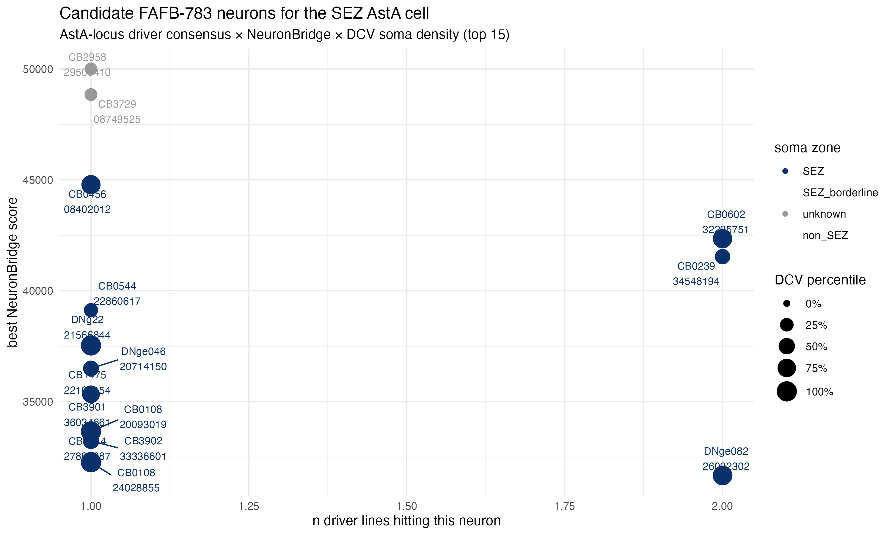
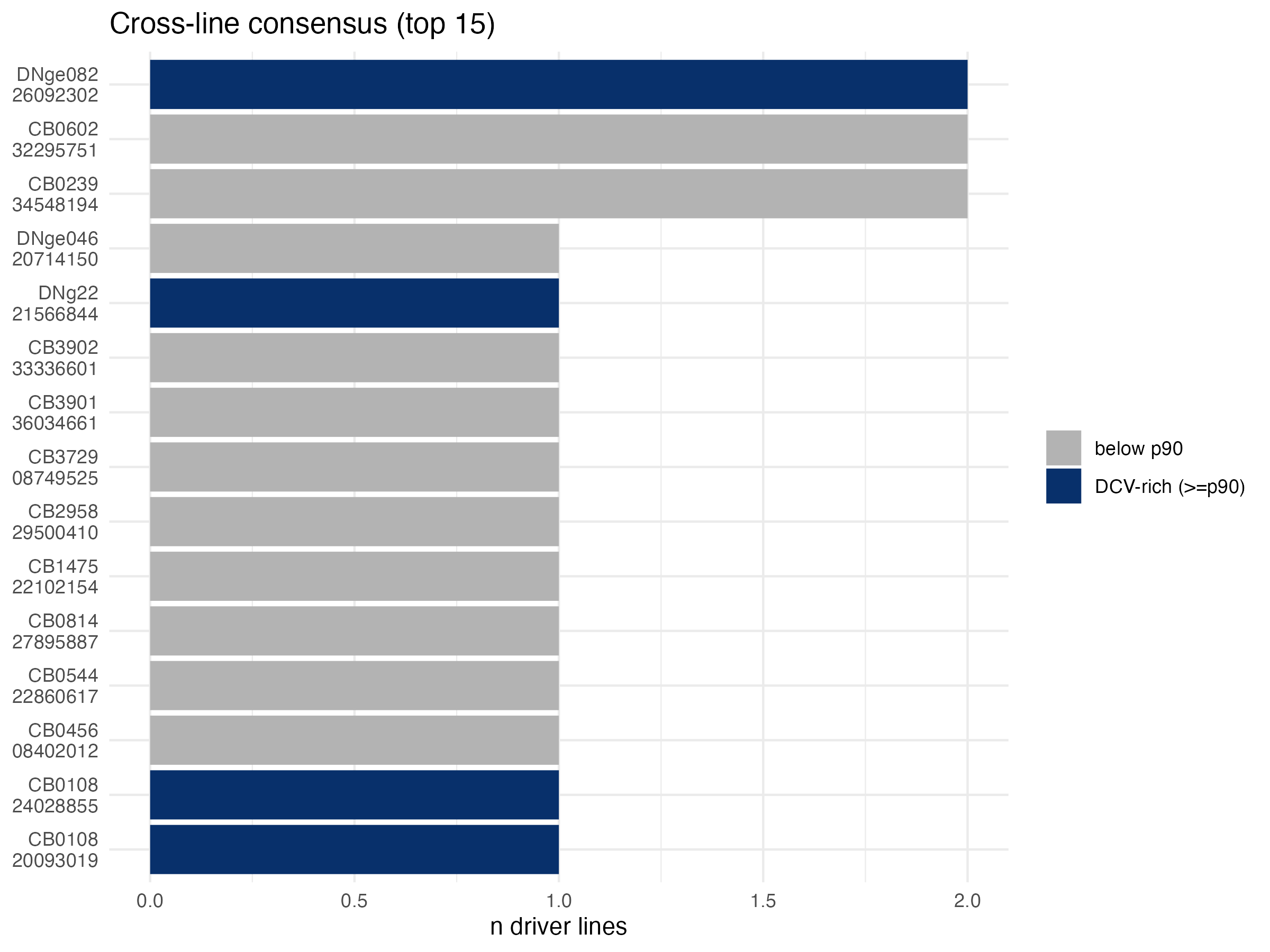
Two graphical summaries — first the dot plot of best NB score versus consensus, second the ranked bar with DCV-rich highlight:
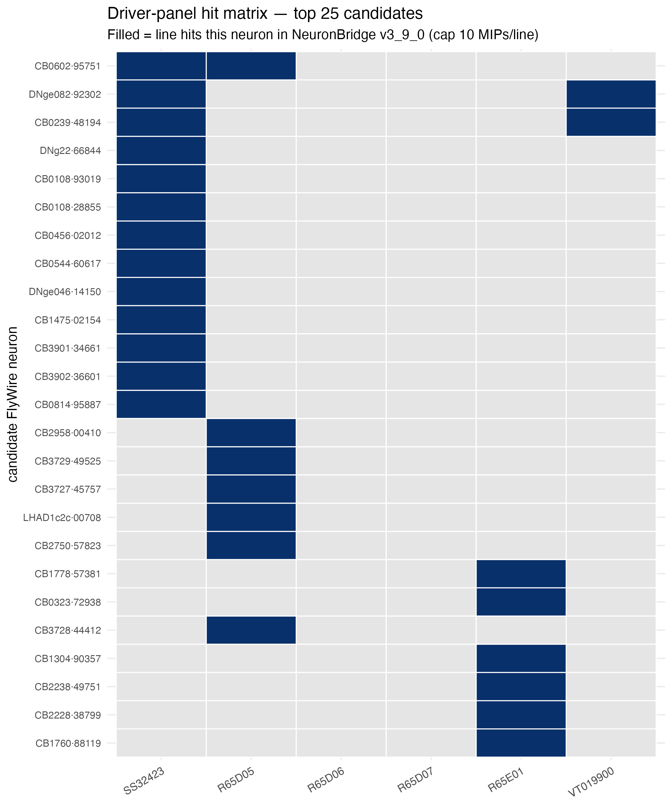
The driver-panel hit matrix shows which of our six AstA-locus drivers hit each top-25 candidate — useful for seeing at a glance who’s a consensus winner and who’s a one-line hit:
Step 7: Reading the table — what do these candidates mean?
A few things stand out:
-
CB0602is the only neuron hit by both SS32423 and R65D05 (the canonical AstA-GAL4) at high score. It’s acentral_brain_intrinsiccell with soma in the SEZ (frac_sez = 1.0),putative_primaryhemilineage, predicted ACh, anddcv_pct = 0.866(just below the strict p90 DCV-rich threshold). This is the strongest candidate for the SS32423 SEZ AstA neuron. FlyWire root720575940632295751. -
CB0239(LB11hemilineage, ACh,dcv_pct = 0.402) is hit by both SS32423 andVT019900(SS32423’s AD half). Lower DCV signal, butLB11is an SEZ-relevant lineage. Worth visually verifying. FlyWire root720575940634548194. -
DNg22turns up in SS32423 alone — confirmednp_verified = "FMRFa", very DCV-rich (dcv_pct = 1.0,soma_dcv_density = 50.1). This is a known peptidergic descending neuron rather than the canonical Hergarden-type SEZ AstA cell, but the SS32423 colour-MIP almost certainly contains the DNg22 dendritic arbour and that’s why it ranks. Treat as a secondary hit, not the target. - A cluster of central-brain intrinsic cells in SEZ-relevant
hemilineages (CB1475 in
LB23, CB3901 inMX0__prim, CB3902 inLB0_anterior, CB0456 / CB0544 inputative_primary) sit in the next rank tier. These are all SEZ-soma cells with various NTs and mid-range DCV percentiles — worth a 3-D look for any morphology match. -
DNge046(descending inLB5__prim, gaba,dcv_pct = 0.437) is the second descending neuron in the candidate set after DNg22. Like DNg22 it’s likely arbour-overlap rather than the AstA cell. - The 16 SS32423 hits with non-SEZ somas (visible in
asta_sez_ranked_full.csv) include cells in SMP / SLP / LH cortex rinds — these are off-target SS32423 labelling, not the AstA cell. We keep them in the CSV for transparency but they fall out of the SEZ-OK figures.
The ranked CSV with all 100+ candidates and full annotations is in
inst/extdata/asta_sez/asta_sez_ranked_full.csv. The top-30
cut is asta_sez_ranked_top30.csv.
Step 8: Visualise the top two candidates with
nat.ggplot
nat.ggplot::geom_neuron() plots a neuron /
neuronlist / mesh as a 2-D ggplot — the same idiom the
lee-lab DCV repo uses for its FAFB figures
(R/visualise/fafb_flange.R,
fig_2_dcv_predictions_fafb.Rmd). We fetch the L2 skeletons
of the top 2 candidates from FlyWire, then overlay them on the FAFB14
brain with the SEZ neuropils tinted blue:
library(nat); library(nat.ggplot); library(elmr); library(fafbseg)
library(ggplot2); library(patchwork)

CB0602 <- "720575940632295751"
CB0239 <- "720575940634548194"
sk <- read_l2skel(c(CB0602, CB0239),
                  datastack_name = "flywire_fafb_public")

brain    <- elmr::FAFB14.surf
sez_surf <- subset(elmr::FAFB14NP.surf,
                   c("GNG","SAD","FLA_R","FLA_L","AMMC_R","AMMC_L"))

mk_panel <- function(neuron, title, neuron_col) {
  ggplot() +
    geom_neuron(brain,    cols = "grey70", alpha = 0.35) +
    geom_neuron(sez_surf, cols = "#3182bd", alpha = 0.45) +
    geom_neuron(neuron,   cols = neuron_col, alpha = 0.95, lwd = 0.4) +
    coord_fixed() + scale_y_reverse() + guides(colour = "none", fill = "none") +
    labs(title = title) +
    theme_void(base_size = 11) +
    theme(plot.title = element_text(hjust = 0.5))
}
(mk_panel(sk[[CB0602]], "CB0602 — SS32423 ∩ R65D05",   "magenta") |
 mk_panel(sk[[CB0239]], "CB0239 — SS32423 ∩ VT019900", "darkorange"))
The result
(inst/images/asta_sez_candidates_natggplot.png):
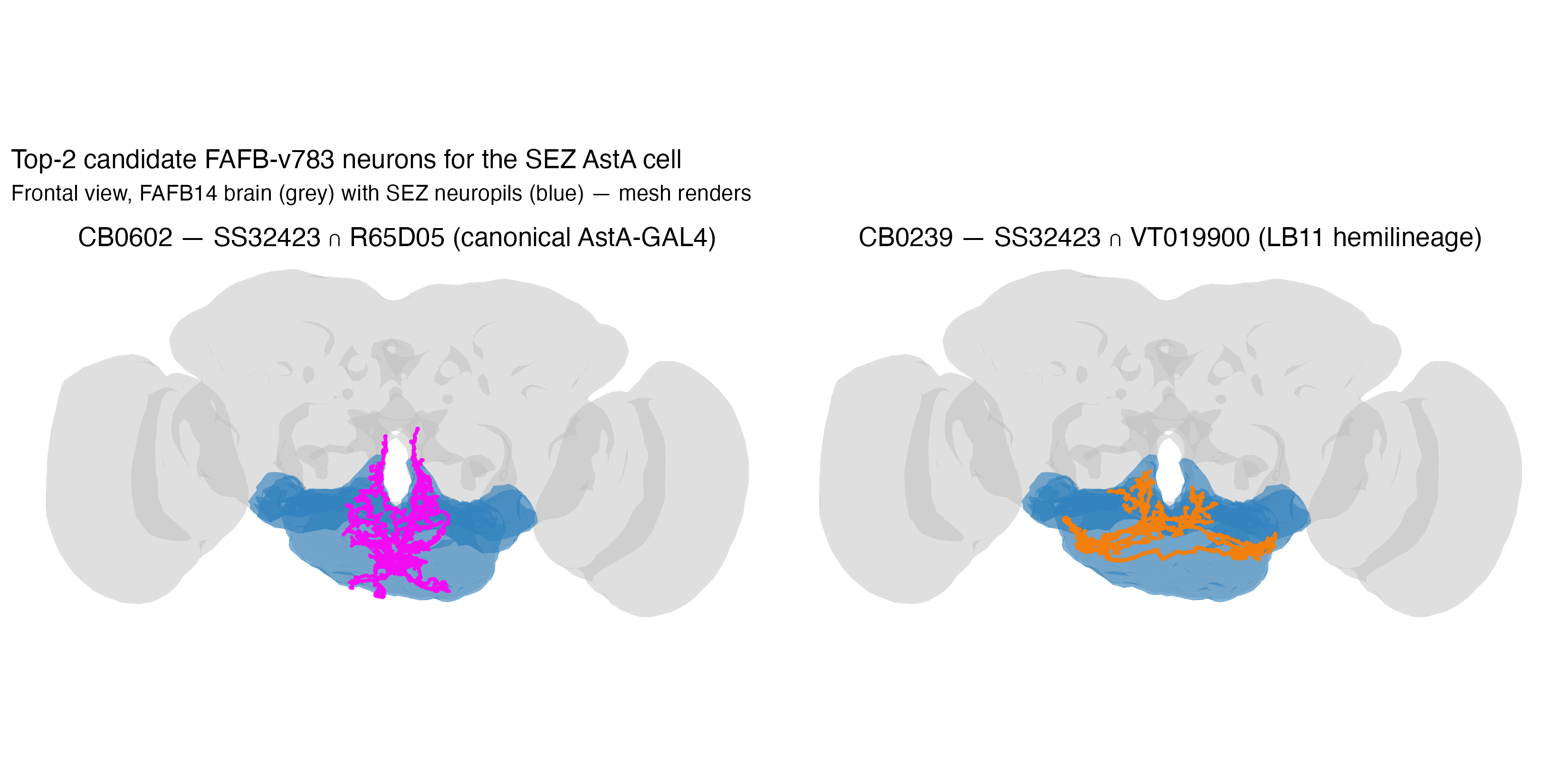
CB0602 has the soma in the SEZ neuropil (left side) and arbours extending dorso-medially into central brain — exactly the bilateral SEZ-soma → SMP-arbour pattern visible across the SS32423 montage. CB0239 is a tighter, more SEZ-local cell.
Step 9: Side-by-side colour-depth MIP
Stack the SS32423 NB brain MIP next to depth-encoded renders of CB0602 and CB0239 (using the same blue→cyan→green→yellow→orange→red→magenta ramp NeuronBridge uses), so the three panels read consistently:
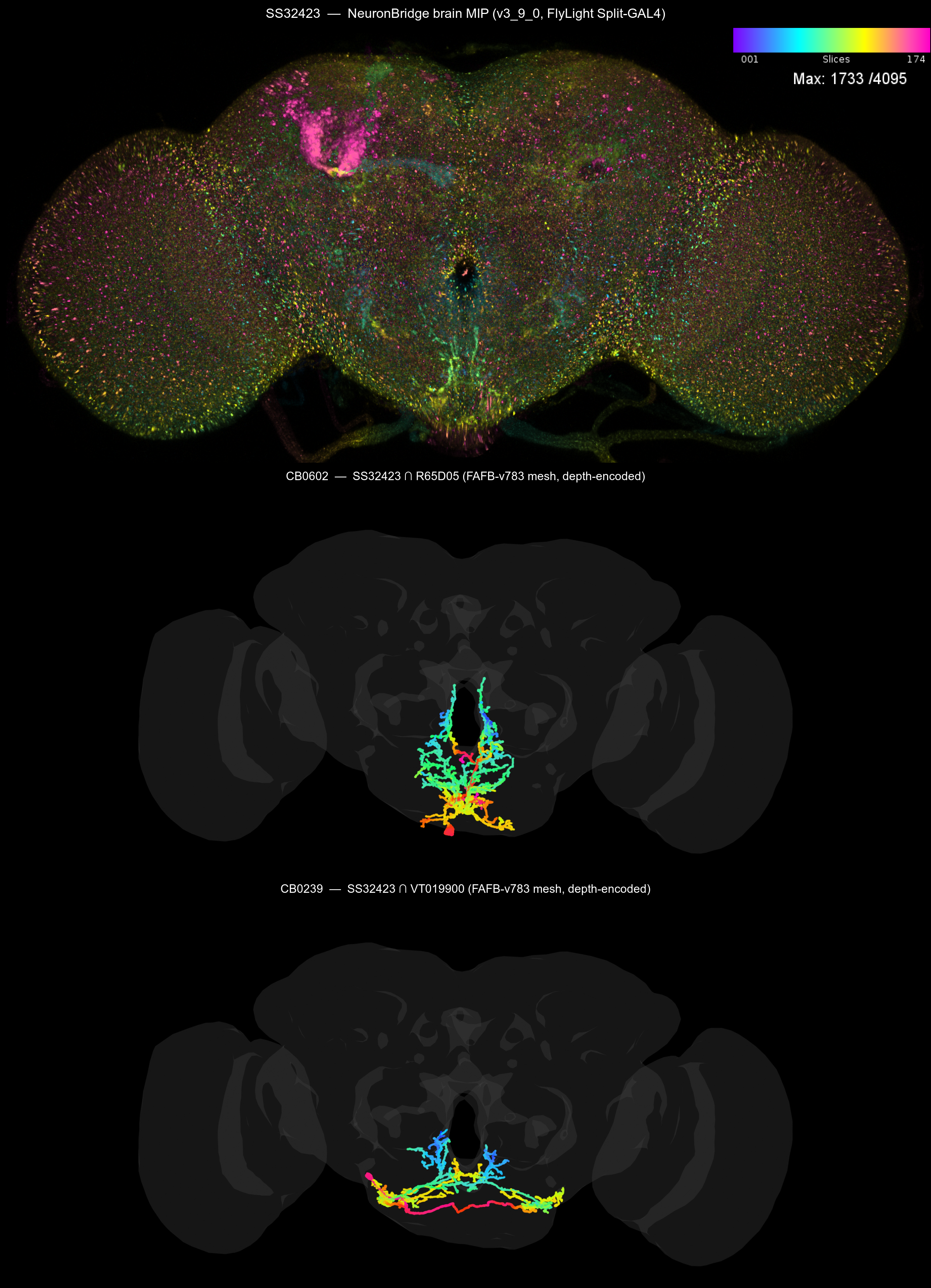
The reproducer for this figure (and the geom_neuron
panel above) is inst/scripts/asta_sez_mip_panel.R and
inst/scripts/asta_sez_natggplot.R — both run from L2
skeletons (fast, ~20 s for 2 neurons) rather than full meshes.
If you want a true NeuronBridge-style colour-depth MIP from
the FlyWire mesh (i.e. Janelia’s
Color_Depth_MIP_batch_0308_2021.ijm macro applied to a
re-rendered NRRD), the package wraps that pipeline too — but it needs a
working FAFB CloudVolume + FIJI/CMTK install:
root_id_to_nrrd("720575940632295751",
                reference  = "JRC2018U_HR",
                savefolder = "~/asta_sez_mips")
nrrd_to_mip(fiji.path = "/Applications/Fiji.app/Contents/MacOS/ImageJ-macosx",
            savefolder = "~/asta_sez_mips")
Where that’s unavailable, the BANC
colormips pure-Python pipeline produces visually
compatible output without FIJI.
Caveats
- SS32423 is a “weak” labeller of the AstA SEZ neuron — the colour-depth scores are only mid-range, and the bright cell at the top of the SS32423 MIP is a different (stronger) cell of the line’s pattern. Trust the visual MIP / 3-D match, not the rank order alone.
-
DCV density is a peptidergic proxy, not an AstA-specific
marker. CB0602 sitting at
dcv_pct = 0.866is consistent with peptide release but does not pin down which neuropeptide. Thenp_verifiedcolumn will catch AstA-positive neurons that have already been annotated; absence there is “not yet verified”, not “negative”. -
Soma-neuropil via DCV-vesicle tokenisation is
approximate. Comma-joined boundary labels and the
outside_*rind classes are both included on purpose, andunknown(no soma DCVs) is kept rather than dropped. The hard filter isin_ss32423plus cross-line consensus; soma-zone is a nudge. -
MIP cap = 5/line is a quadratic-cost trade-off.
With more MIPs per line we’d expect more cross-line consensus (currently
only 2 candidates have
n_lines >= 2). If you need that, raise the cap in step 1 and tolerate a longer pipeline run; theinst/extdata/asta_sez/cache/per-line.rdsfiles mean a re-run only does the new lines. -
NeuronBridge data version. This vignette is written
against
v3_9_0, the first release with the corrected FlyWire-v783 alignment. Earlier releases will give worse top-N hit lists. -
AstA drivers not in NeuronBridge.
P{AstA-GAL4.2.1}(Hentze 2015),AstA[SK1]CRISPR, MiMIC T2A-GAL4 — all not in NB and so cannot contribute to the consensus here. -
Hemidriver self-reinforcement. SS32423’s two halves
are themselves AstA-locus enhancers and appear in the panel — i.e. the
cross-line consensus partly self-reinforces. This is fine for finding
the AstA cell, but the test for “is this an AstA neuron?” is whether
R65D05(the canonical AstA-GAL4) hits it, not just whether SS32423’s halves do. By that test, CB0602 wins.
Iteration
If the visual MIP / 3-D comparison shows CB0602 doesn’t match SS32423, three knobs to turn in order:
-
Raise the per-line MIP cap from 10 (e.g. to 20) —
the strongest candidates with
n_lines >= 2will probably remain, but broader consensus will surface ties we missed. Bear in mindneuronbridge_hits()usesplyr::rbind.fillinternally and is quadratic in result rows, so cap=20 across the panel is roughly 3× slower than cap=10. -
Drop the
R65D07/R65E01flanking tiles — these contribute many off-target consensus hits that aren’t in theR65D05∩SS32423intersection (visible asR65E01-only andR65D07-only stripes on the heatmap). A tighter panel (SS32423,R65D05,R65D06,VT019900) privileges AstA-specific enhancers over locus-wide ones. -
Re-rank without the DCV nudge — CB0602 sits at
dcv_pct = 0.866, just below the strict p90 cutoff, so the nudge isn’t helping it; if the true AstA cell sits even lower in DCV, the nudge could be pushing the wrong cell to the top.
Citations
- NeuronBridge: Clements, J., Goina, C., Kazimiers, A., Otsuna, H., Svirskas, R., Rokicki, K. (2020). NeuronBridge Codebase.
- SS32423 / aMulet: Sterne, G.R., Otsuna, H., Dickson, B.J., Scott, K. (2021). eLife 10:e71679.
- AstA-GAL4 (R65D05): Hergarden, A.C., Tayler, T.D., Anderson, D.J. (2012). PNAS 109(10):3967–3972.
- AstA in feeding circuits: Pool, A.-H. et al. (2014). Neuron 83(1):164–177.
- Janu-AstA / thirst: Landayan, D., Wang, B.P., Zhou, J., Wolf, F.W. (2021). eLife 10:e66286.
- AstA biology: Chen, J. et al. (2016) PLoS Genet 12(8):e1006346; Hentze, J.L. et al. (2015).
- FlyWire / FAFB-v783: Dorkenwald, S. et al. (2024); Schlegel, P. et al. (2024). Nature.
-
DCV detection / soma DCV density: lee-lab DCV
manuscript (in preparation; methodology in
/Users/GD/LMBD/Papers/dcv).