Symmetrising the L1 larval CNS and finding left-right cognates

Goal

The L1 larval connectome — the first-instar Drosophila larval CNS, manually reconstructed and hosted openly by Virtual Fly Brain — is very nearly bilaterally symmetric. This vignette builds a left-right symmetrising diffeomorphism for the whole L1 CNS (brain and ventral nerve cord) from its matched left/right neuropil compartments, uses it to carry structures across the midline onto their contralateral partners, and then finds cognate neuron pairs by morphological similarity (NBLAST) once the two sides are in register.

Ten years ago this package was an L1-only tool: it shipped hard-wired helpers — apply_mirror_affine(), symmetrise_l1(), other_side() for the symmetrising map, and find_cognate() / check_l1_cognates() for the left-right cognate search — each backed by a bundled transform and a bespoke L1 NBLAST scoring matrix. deformetricar is no longer L1-specific, so those functions are gone from the package. This vignette rebuilds them from scratch, as a few lines each over the general deformetricar (and nat.nblast) API, driven by the live VFB dataset. That is the point of the walkthrough: the five functions are the deliverable.

The right Kenyon cells (rose) sweeping across the midline onto their left cognates (blue) under the symmetrising map — their somata drawn as circles — over the static grey L1 CNS, viewed along the head-to-tail long axis.

library(deformetricar)
library(nat)
library(catmaid)          # aka rcatmaid
library(Rvcg)             # mesh clean / decimate
library(Morpho)           # applyTransform

1. Acquire the L1 data from Virtual Fly Brain

The L1 larval CATMAID is public and read-only — no login needed. Connect once; from there everything is a query against that connection. We pull two kinds of object: the neurons (fetched by annotation) and the neuropil compartment volumes that will anchor the symmetrising warp.

l1 <- catmaid_connection(server = "https://l1em.catmaid.virtualflybrain.org/")
# Deformetrica needs ~O(1-100) coordinates: work in um, not the raw nm.
nm2um <- function(x) { xyzmatrix(x) <- xyzmatrix(x) / 1000; x }

The neurons

Cells are fetched by annotation. The L1 dataset is richly annotated — browse the tags with catmaid_get_annotationlist(conn = l1) — so a query like "annotation:Kenyon Cell right" returns every skeleton tagged with it. get_neurons() fetches an annotation’s skeletons, resamples them and puts them in µm; we take the left and right Kenyon cells as a clean, bilaterally-matched test set. Swap the annotation for any cell type, or widen it to pull the whole ~4,000-neuron CNS.

get_neurons <- function(ann, n = NULL) {
  x <- read.neurons.catmaid(catmaid_skids(ann, conn = l1), conn = l1)
  x <- nat::nlapply(nat::nlapply(x, nat::resample, stepsize = 1500), nm2um)
  if (!is.null(n) && length(x) > n) x[round(seq(1, length(x), length.out = n))] else x
}
KCR <- get_neurons("annotation:Kenyon Cell right")   # all right Kenyon cells
KCL <- get_neurons("annotation:Kenyon Cell left")    # all left  Kenyon cells

The CNS surface and its left/right compartments

The dataset also ships the whole-CNS surface (cns) plus a set of bilateral neuropil volumes — the two brain hemispheres, the SEZ, and the thoracic/abdominal VNC segments (T1–T3, A1–A8), each as a _left/_right pair. Those matched pairs are the anchors that teach the warp what “symmetric” means; we take a spread of them down the whole length of the CNS.

vl <- catmaid_get_volumelist(conn = l1)
get_volume <- function(name) nm2um(Rvcg::vcgClean(
  as.mesh3d(catmaid_get_volume(vl$id[vl$name == name], conn = l1, rval = "mesh3d")),
  sel = 0, silent = TRUE))

cns   <- get_volume("cns")                                    # the whole CNS surface
pairs <- c("Brain Hemisphere", "SEZ", "T1", "T2", "A3", "A6")   # head -> tail spread
lname <- function(p) if (p == "Brain Hemisphere") "Brain Hemisphere left"  else paste0(p, "_left")
rname <- function(p) if (p == "Brain Hemisphere") "Brain Hemisphere right" else paste0(p, "_right")
L <- setNames(lapply(pairs, function(p) get_volume(lname(p))), pairs)
R <- setNames(lapply(pairs, function(p) get_volume(rname(p))), pairs)

2. `apply_mirror_affine()` — reflect one side onto the other

The linear half of a symmetrising map. Reflect an object across the CNS midline plane (so left ↔︎ right), then rigidly affine-align that reflection back onto the original CNS — this removes the fact that the specimen’s midline is neither exactly at x = 0 nor exactly axis-aligned. Everything downstream rides this same transform, so we fit it once (from the whole CNS) and wrap it as a function.

midX   <- mean(range(xyzmatrix(cns)[, 1]))                # specimen midline (x)
mirror <- function(m) {                                   # reflect across x = midX
  xyzmatrix(m)[, 1] <- 2 * midX - xyzmatrix(m)[, 1]
  if (!is.null(m$it)) m$it <- m$it[c(2, 1, 3), ]          # keep surface winding outward
  m$normals <- NULL; m
}
pre <- affine_prealign(mirror(cns), cns, type = "rigid")  # reflection -> original CNS

# apply_mirror_affine(x): reflect x, then apply that same rigid alignment.
apply_mirror_affine <- function(x) pre$apply(mirror(x))

3. Fit the symmetrising diffeomorphism from the matched compartments

The affine cannot capture the specimen’s non-rigid left-right asymmetry (a slightly bent VNC, one hemisphere fuller than the other). A diffeomorphism can. We fit one diffeomorphism to the whole set of matched compartments at once with deformetrica_register_multi(), in both directions so the result is genuinely symmetric: each mirror-affined right compartment is driven onto its left partner, and each mirror-affined left onto its right. Registering the compartment surfaces (not the ~thousands of neurons) is what keeps this cheap and robust.

dec  <- function(m, n = 700L) Rvcg::vcgQEdecim(m, tarface = n)
srcs <- tgts <- list()
for (p in pairs) {
  srcs[[paste0(p, "_R")]] <- dec(apply_mirror_affine(R[[p]])); tgts[[paste0(p, "_R")]] <- dec(L[[p]])
  srcs[[paste0(p, "_L")]] <- dec(apply_mirror_affine(L[[p]])); tgts[[paste0(p, "_L")]] <- dec(R[[p]])
}
kw  <- sqrt(sum((apply(xyzmatrix(cns), 2, max) - apply(xyzmatrix(cns), 2, min))^2)) / 12
fit <- deformetrica_register_multi(srcs, tgts, kernel_width = kw, data_sigma = 3,
                                   timepoints = 15L, max_iterations = 40L, device = "auto")

4. `symmetrise_l1()` and `other_side()` — the full contralateral map

Now compose the two halves. symmetrise_l1() mirror-affines an object and then flows it through the fitted diffeomorphism — the complete non-linear symmetrisation. Because the diffeomorphism that makes the CNS symmetric is exactly the map that carries each structure onto its contralateral partner, other_side() — “send this neuron to the other side of the CNS” — is the very same function. (flow = TRUE keeps every geodesic timepoint, for the animation; the default returns just the endpoint.)

symmetrise_l1 <- function(x, flow = FALSE)         # `fit` is a portable `deformetricareg`
  deformetrica_shoot(apply_mirror_affine(x), fit, flow = flow)

other_side <- symmetrise_l1        # the symmetrising map IS the left<->right map

These three functions — apply_mirror_affine(), symmetrise_l1(), other_side() — are the modern, dataset-driven replacements for the old bundled helpers. They accept anything with xyzmatrix() coordinates: a points matrix, a mesh3d, a neuron or a neuronlist.

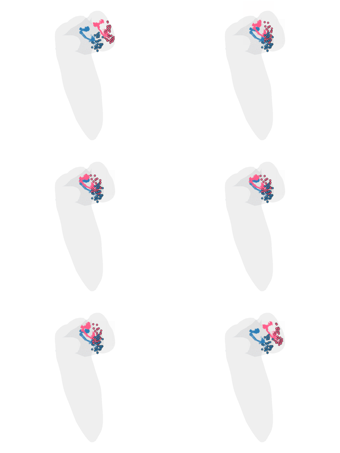
5. Watch the map carry the right cells onto their left cognates

The whole L1 CNS is so nearly symmetric that the surface deformation is only a few µm — true to the biology, but too subtle to watch. The striking thing to see is the map applied to cells: send the right Kenyon cells across the midline with other_side() and watch them land on their left partners. We animate the full journey in two acts — the mirror-affine reflection (a big, ~50 µm cross-midline sweep) and then the diffeomorphic flow — over a static grey CNS, viewed along its long axis (first principal component, head-to-tail) so the bilateral symmetry is edge-on. The left Kenyon cells (blue) are drawn static as the target the right ones (rose) should meet.

# a legible subset of the KCs fetched in §1, so the animation is not too dense
sub36 <- function(x) x[round(seq(1, length(x), length.out = min(36, length(x))))]
kcR <- sub36(KCR); kcL <- sub36(KCL)

# the two acts of other_side(): the mirror-affine sweep, then the diffeomorphic flow
interp  <- function(o, from, to, n) lapply(seq(0, 1, length.out = n),
             function(a) { x <- o; xyzmatrix(x) <- (1 - a) * from + a * to; x })
aff_kc  <- apply_mirror_affine(kcR)                                    # reflect + rigid
act1    <- interp(kcR, xyzmatrix(kcR), xyzmatrix(aff_kc), 12)          # the cross-midline sweep
act2    <- deformetrica_shoot(aff_kc, fit, flow = TRUE)                # the diffeomorphism
flow_kc <- c(act1, act2)

# each Kenyon cell is rooted at its soma, so its root point IS the cell body: draw
# those as circles (the moving right somata, the static left ones) with `points`.
soma_of <- function(nl) do.call(rbind, lapply(nl, function(n) xyzmatrix(n)[nat::rootpoints(n)[1], , drop = FALSE]))
somata_R <- lapply(flow_kc, soma_of)          # per-frame, move with the sweep
somata_L <- soma_of(kcL)                       # static targets

# view: long axis (PC1) vertical, next axis horizontal, shortest into the screen
pc <- prcomp(xyzmatrix(cns))$rotation
RM <- diag(4); RM[1, 1:3] <- pc[, 2]; RM[2, 1:3] <- -pc[, 1]; RM[3, 1:3] <- pc[, 3]
ggplot_flow_gif(list(KC_right = flow_kc),
                cols = list(KC_right = "#FF5C8A"), alpha = c(KC_right = 0.35),
                targets = list(KC_left = kcL), target_cols = c(KC_left = "#2C7FB8"),
                target_alpha = 0.28,
                points = list(KC_right = somata_R, KC_left = somata_L),
                point_cols = c(KC_right = "#FF5C8A", KC_left = "#2C7FB8"),
                point_size = 3, point_alpha = 0.85,
                volume = cns, volume_col = "grey65", volume_alpha = 0.10,
                rotation_matrix = RM, delay = 0.12,
                file = "l1_symmetrise.gif")   # somata as circles; grey CNS + left KCs as context

6. `find_cognate()` and `check_l1_cognates()` — the cognate search

With a symmetrising map, cognate-finding is direct: send every right neuron across with other_side(), then NBLAST it against the left neurons — the top hit is its putative left cognate. Two choices make this L1-tuned, as the original was: UseAlpha = TRUE (which up-weights each neuron’s tract-like backbone), and an L1-scale scoring matrix. NBLAST’s default matrix is trained on the adult fly, whose neurons are an order of magnitude larger; the L1 matrix bins distances from fractions of a micron (its first breaks are 0.75, 1.5 µm, versus 2.5 µm for the adult), so L1 near-misses are scored on the right scale. Build one from provisional cognate pairs with nat.nblast::create_scoringmatrix() at those L1 distbreaks; here we pass the adult alpha matrix smat_alpha.fcwb to keep the walkthrough self-contained.

library(nat.nblast)
dp <- function(nl) nat::dotprops(nl, resample = 0.5, k = 5, .progress = "none")

# find_cognate(x, db_dps): carry x across with other_side(), NBLAST against the
# contralateral database, return each neuron's ranked cognates with scores.
find_cognate <- function(x, db_dps, smat = smat_alpha.fcwb, n = 5) {
  q  <- dp(other_side(x))
  sc <- nblast(q, db_dps, smat = smat, normalised = TRUE, UseAlpha = TRUE, .progress = "none")
  lapply(stats::setNames(colnames(sc), colnames(sc)), function(j) {
    o <- order(sc[, j], decreasing = TRUE)[seq_len(n)]
    data.frame(cognate = rownames(sc)[o], score = round(sc[o, j], 3))
  })
}

kcl_dps <- dp(KCL)                                 # KCR / KCL were fetched in §1

cog <- find_cognate(KCR, kcl_dps)                  # ranked left cognates per right KC
cog[[1]]                                           # top-5 cognates + scores for one right KC

Reciprocal best hits. A cognate call is trustworthy when the two neurons are each other’s top match both ways — right→left and left→right agree. That mutual-best-hit set is the confident left-right mapping, and its size is a clean score for the whole symmetrisation.

top1 <- function(res) vapply(res, function(d) d$cognate[1], character(1))
r2l  <- top1(find_cognate(KCR, kcl_dps))                       # right skid -> best left skid
l2r  <- top1(find_cognate(KCL, dp(KCR)))                       # left  skid -> best right skid
rbh  <- names(r2l)[l2r[r2l] == names(r2l)]                    # mutual top-1 pairs
sprintf("%d / %d right Kenyon cells have a reciprocal-best-hit left cognate",
        length(rbh), length(r2l))

check_l1_cognates() — the old interactive rgl inspector, as a static nat.ggplot panel: a right query carried across the midline (rose) over its top-ranked left cognate (blue), viewed along the CNS long axis (the RM from §5).

check_l1_cognates <- function(right_skid, db_right, db_left, cog, RM) {
  q    <- other_side(db_right[right_skid])
  best <- db_left[cog[[right_skid]]$cognate[1]]
  ggplot2::ggplot() +
    nat.ggplot::geom_neuron(q,    rotation_matrix = RM, cols = c("#FF5C8A", "#FF5C8A")) +
    nat.ggplot::geom_neuron(best, rotation_matrix = RM, cols = c("#2C7FB8", "#2C7FB8")) +
    ggplot2::coord_fixed() + ggplot2::theme_void()
}
check_l1_cognates(names(rbh)[1], KCR, KCL, cog, RM)   # inspect the first confident pair

The original ran this over the whole L1 CNS — all ~4,000 reconstructed neurons at once, not just the Kenyon cells — to build a left-right map for the entire connectome. find_cognate() scales straight to that: pass the whole-CNS dotprops as db_dps.

Notes

Why compartments, not neurons, drive the fit. Registering a handful of decimated compartment surfaces is cheap and numerically stable; fitting to thousands of neuron skeletons at once is neither. The neurons are what we apply the finished map to — that is always cheap (deformetrica_shoot()).
The five functions are the point. apply_mirror_affine(), symmetrise_l1(), other_side(), find_cognate() and check_l1_cognates() are just closures over pre, fit and (for the search) a scoring matrix. Swap the dataset (or the compartment list) and you have a symmetriser + cognate-finder for any other nervous system — nothing here is L1-specific any more, which is exactly why they no longer live in the package.
L1-scale NBLAST. The original shipped a bespoke L1 scoring matrix because the default is trained on adult-fly neurons ~10× larger; on L1 you want distance bins that start below a micron. UseAlpha = TRUE matters too — Kenyon cells and VNC tracts are near-parallel bundles, and the alpha term rewards that shared backbone geometry.
More anchors, better VNC. Add more of the A1–A8 / T1–T3 pairs to pairs for a tighter fit along the nerve cord; the original also drove the warp with named fibre tracts (the antennal-lobe tracts, the dorso/ventro-medial/lateral VNC tracts) as extra matched anchors — add any bilateral pair you can name to srcs/tgts.