Plot neurotransmitter prediction summaries or synapses in 3D

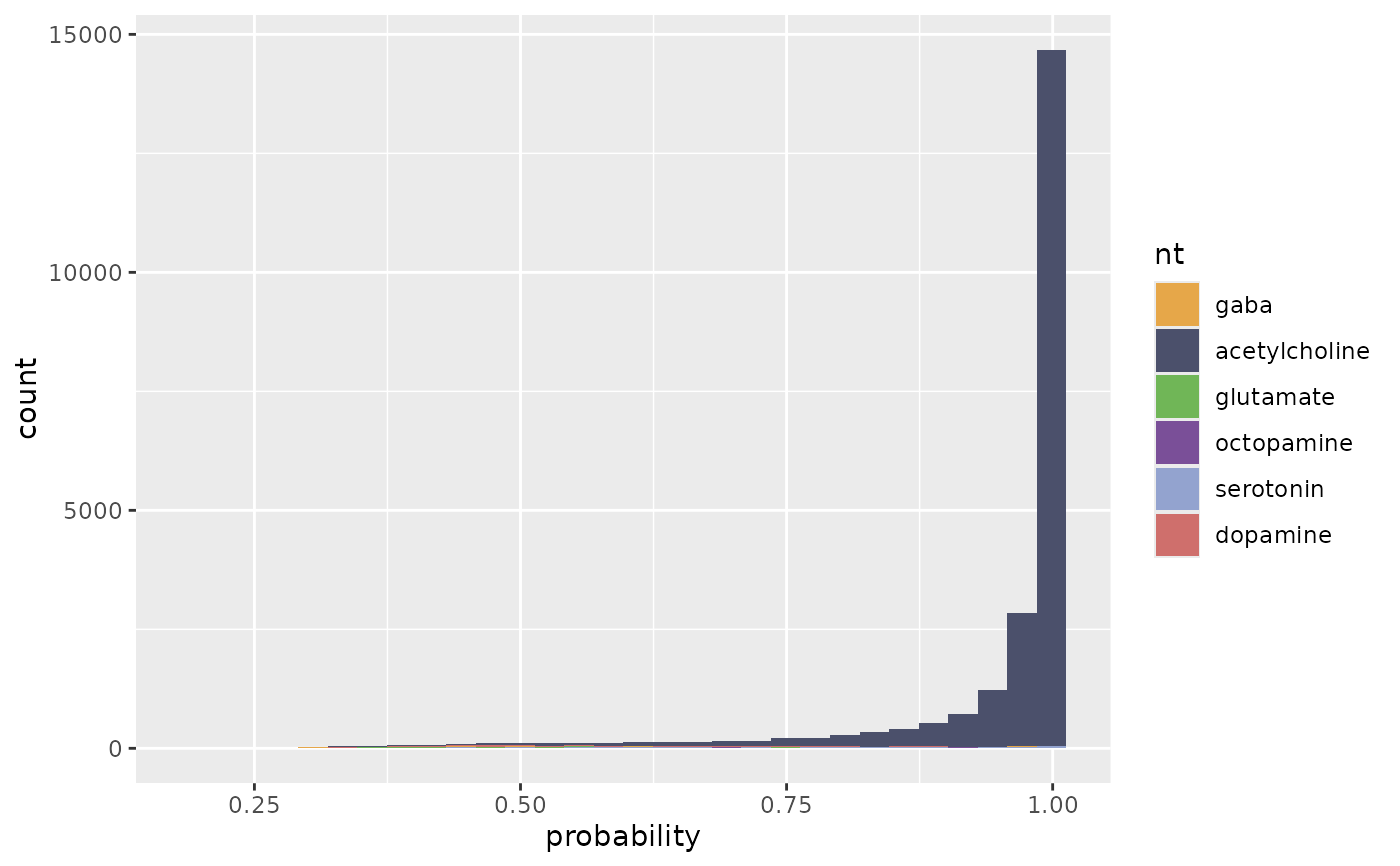
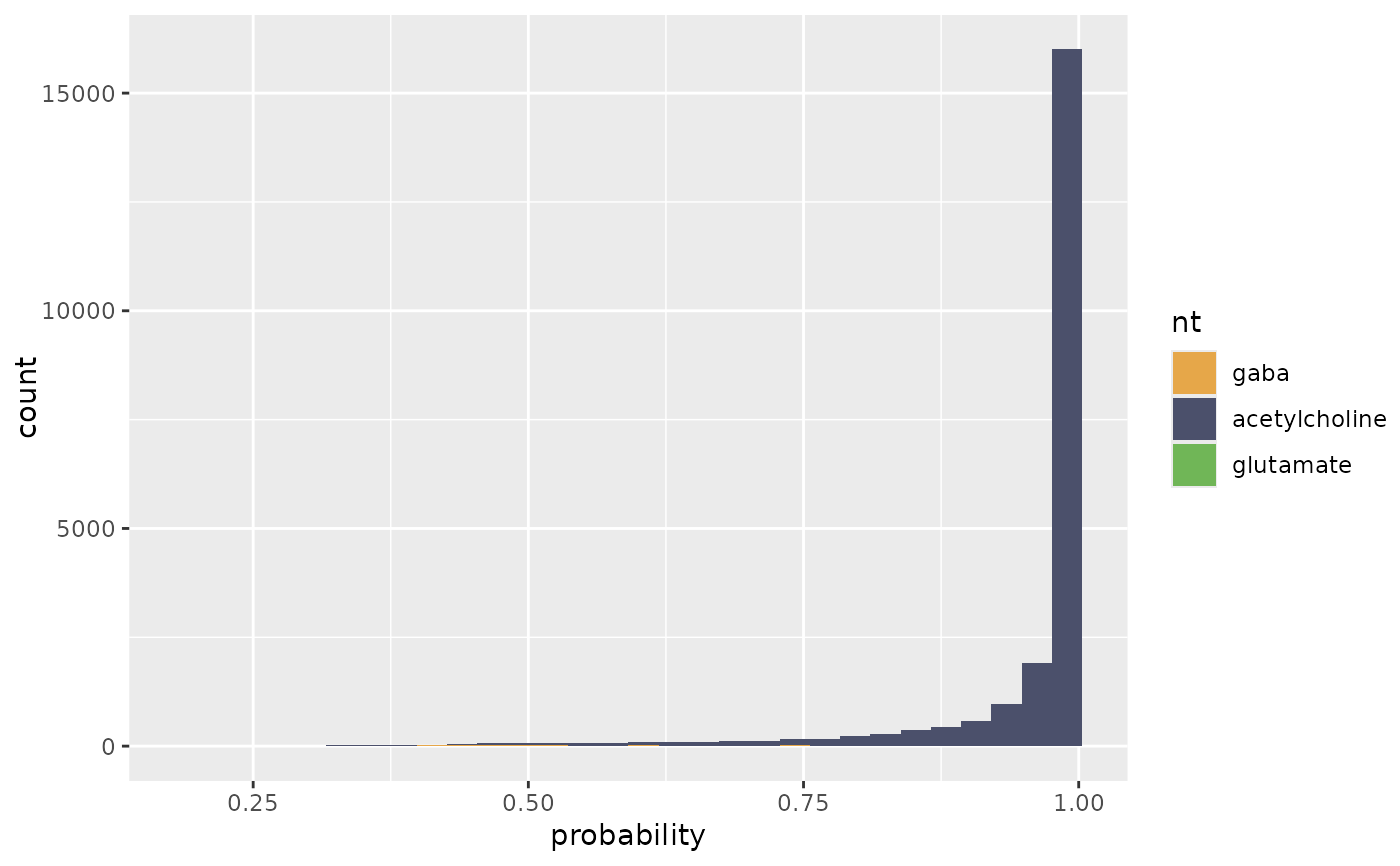
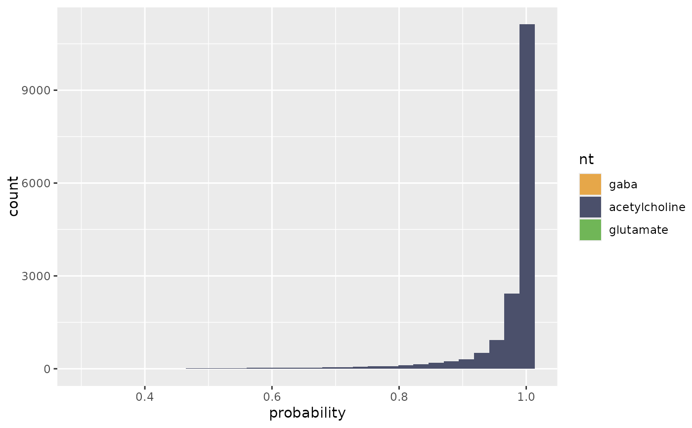
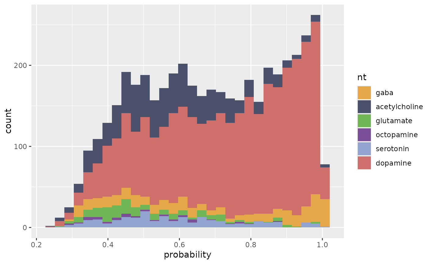
flywire_ntplot plots a ggplot2 histogram of predicted neurotransmitter vs prediction probability.

flywire_ntplot3d makes a 3D plot of synapse location

Usage

flywire_ntplot(
  x,
  nts = c("gaba", "acetylcholine", "glutamate", "octopamine", "serotonin", "dopamine",
    "neither"),
  cleft.threshold = 0,
  local = NULL,
  cloudvolume.url = NULL
)

flywire_ntplot3d(
  x,
  nts = c("gaba", "acetylcholine", "glutamate", "octopamine", "serotonin", "dopamine"),
  plot = c("points", "spheres"),
  cleft.threshold = 0,
  local = NULL,
  cloudvolume.url = NULL,
  ...
)

Arguments

x

A flywire rootid or a data.frame of neurotransmitter predictions returned by flywire_ntpred

nts

A character vector of neurotransmitters to include in the plot (default all 6)

cleft.threshold

A threshold for the cleft score calculated by Buhmann et al 2019 (default 0, we have used 30-100 to increase specificity)

local

path to SQLite synapse data. Evaluated by fafbseg:::local_or_google. Work in progress. Default is to download this data and place it in ~/projects/JanFunke.

cloudvolume.url

The segmentation source URL for cloudvolume. Normally you can ignore this and rely on the default segmentation chosen by choose_segmentation

plot

Whether to plot points or spheres ("points" with size=5 works quite well)

...

additional arguments passed to spheres3d or points3d

Value

flywire_ntplot returns a ggplot2::ggplot object that can be further customised to modify the plot (see examples).

See also

Other automatic-synapses: flywire_adjacency_matrix(), flywire_neurons_add_synapses(), flywire_ntpred(), flywire_partners()

Examples

# \donttest{
# a cholinergic olfactory projection neuron
ntp=flywire_ntpred("720575940615237849")
#> Warning: /home/runner/projects/JanFunke//flywire_synapses.db does not exist
#> Warning: /home/runner/projects/JanFunke//20191211_fafbv14_buhmann2019_li20190805_nt20201223.db does not exist
flywire_ntplot(ntp)
#> `stat_bin()` using `bins = 30`. Pick better value with `binwidth`.

flywire_ntplot(ntp, nts=c("gaba", "acetylcholine", "glutamate"))
#> `stat_bin()` using `bins = 30`. Pick better value with `binwidth`.

flywire_ntplot(ntp, nts=c("gaba", "acetylcholine", "glutamate"), cleft.threshold=100)
#> `stat_bin()` using `bins = 30`. Pick better value with `binwidth`.


# ids for several Kenyon cells
kcsel=c("720575940623755722", "720575940609992371", "720575940625494549",
"720575940619442047", "720575940620517656", "720575940609793429",
"720575940617265029", "720575940631869024", "720575940637441955",
"720575940638892789")
kcpreds=flywire_ntpred(kcsel)
#> Warning: /home/runner/projects/JanFunke//flywire_synapses.db does not exist
#> Warning: /home/runner/projects/JanFunke//20191211_fafbv14_buhmann2019_li20190805_nt20201223.db does not exist
# collect the ggplot object
p <- flywire_ntplot(kcpreds)
# print it to see the aggregate plot (all neurons together)
p
#> `stat_bin()` using `bins = 30`. Pick better value with `binwidth`.

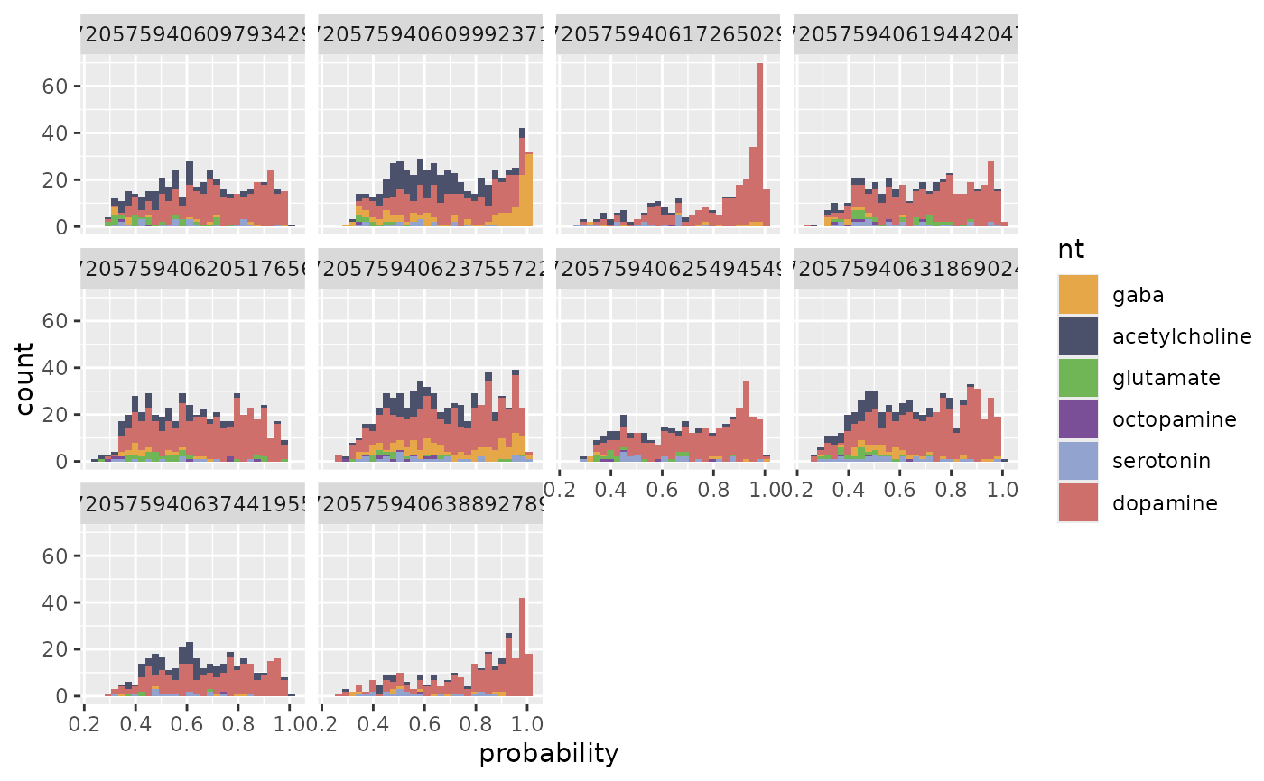
# ... or use ggplot facets to separate by query neuron
p+ggplot2::facet_wrap(query~.)
#> `stat_bin()` using `bins = 30`. Pick better value with `binwidth`.

# }
if (FALSE) { # \dontrun{
flywire_ntplot3d(ntp, nts=c("gaba", "acetylcholine",
  "glutamate"), plot='points', cleft.threshold=30, size=5)
} # }