Colour-depth MIPs from a connectome neuron (BANC AstA1) in JRC2018U_HR
Source:vignettes/colormip_direct_vs_fiji.Rmd
colormip_direct_vs_fiji.RmdOne function, three back-ends
NeuronBridge searches operate on colour-depth MIPs
(Otsuna et al. 2018, bioRxiv): a
single 2-D image where the hue at each (x, y) pixel encodes
the z-depth of the brightest voxel along that column (blue =
anterior, red = posterior).
neuronbridger ships one function —
nrrd_to_mip() — that produces these images via three
interchangeable back-ends, selected with method =:
method |
Implementation | When to use |
|---|---|---|
"direct" (default)
|
Pure R (which.max along z, LUT lookup) |
The fast path; no JVM, no Python |
"python" |
Stephan Gerhard’s port in fanc.render_neurons.make_colormip,
called via reticulate
|
Validate against the BANC reference |
"fiji" |
Janelia’s Color_Depth_MIP_batch_0308_2021.ijm
macro |
Run the canonical FIJI implementation if you already have it installed |
All three use the same 256-entry depth LUT (PsychedelicRainBow2-like
ramp). The output of "direct" is byte-equivalent to
"python" (modulo the 1/255 RGB rounding from skimage’s HSV
roundtrip), and is visually indistinguishable from the FIJI macro —
Stephan’s own characterisation is “nearly identical, with
sub-percent RGB differences that do not affect downstream NeuronBridge
searches.”
Pipeline overview
The MIP step is the last step of a longer pipeline. Steps 1–3 are identical regardless of which back-end you choose for step 4.
| Step | Function | What it does |
|---|---|---|
| 1 | bancr::banc_read_neuron_meshes() |
Fetch a BANC mesh by seg ID |
| 2 |
bancr::banc_to_JRC2018F() +
nat.templatebrains::xform_brain()
|
Bridge into NeuronBridge-compatible template space |
| 3 |
nat::as.im3d() + nat::write.nrrd()
|
Voxelise the registered mesh into a JRC2018U_HR / JRC2018VNCU-shaped volume |
| 4 | nrrd_to_mip(method = ...) |
Colour-depth MIP via R, Python or FIJI |
Steps 1–3 follow the same template-space conventions as wilson-lab/nat-tech
(hemibrain_to_nrrd, flywireid_to_nrrd): a
NeuronBridge-compatible volume must live in
JRC2018_UNISEX_20x_HR (a.k.a. JRC2018U_HR,
dims 1210 × 566 × 174, voxdims
0.5189 × 0.5189 × 1.0 µm) for brain neurons or
JRC2018_VNC_UNISEX_461 (dims
573 × 1119 × 219, voxdims 0.461 × 0.461 × 0.7
µm) for VNC neurons.
Setup
remotes::install_github("natverse/neuronbridger")
remotes::install_github("flyconnectome/bancr")
remotes::install_github("natverse/nat.flybrains")
remotes::install_github("natverse/nat.jrcbrains")
nat.jrcbrains::download_saalfeldlab_registrations()

# For method = "python":
install.packages("reticulate")
reticulate::py_install(c("banc", "scikit-image", "numpy"), pip = TRUE)Step 1 — Find the AstA1 neuron in BANC
AstA1 is the FlyWire/BANC label for the dorsal
peptidergic ascending pair that the asta_sez
vignette converges on from the SS32423 split-GAL4 line. Browse them in
BANC
codex.
ann   <- bancr::banc_codex_annotations()
asta1 <- subset(ann, cell_type == "AstA1")
asta1$pt_root_id

asta1_id <- asta1$pt_root_id[1]
Step 2 — Fetch and bridge into JRC2018U_HR
banc_mesh <- bancr::banc_read_neuron_meshes(asta1_id)

# BANC -> JRC2018F (BANC-specific bridge, tpsreg)
mesh_jrc2018f <- bancr::banc_to_JRC2018F(banc_mesh, method = "tpsreg",
                                         banc.units = "nm")

# JRC2018F -> JRC2018U (natverse bridge from nat.flybrains)
mesh_jrc2018u <- nat.templatebrains::xform_brain(mesh_jrc2018f,
                                                 sample    = "JRC2018F",
                                                 reference = "JRC2018U")
VNC neurons would replace the two transforms with
banc_to_JRC2018F(..., region = "vnc")followed byxform_brain(..., reference = "JRCVNC2018U"), and step 3 would declare the JRCVNC2018U template.
Step 3 — Voxelise to NRRD at JRC2018U_HR dimensions
JRC2018U_HR <- nat.templatebrains::templatebrain(
  "JRC2018U_HR",
  dims    = c(1210, 566, 174),
  voxdims = c(0.5189, 0.5189, 1.0),
  units   = "microns"
)

points <- nat::xyzmatrix(mesh_jrc2018u)
vol    <- nat::as.im3d(points, JRC2018U_HR)

savefolder <- "~/banc_asta1_mip"
dir.create(savefolder, showWarnings = FALSE)
nrrd_path <- file.path(savefolder, sprintf("AstA1_%s_JRC2018U_HR.nrrd", asta1_id))
nat::write.nrrd(vol, nrrd_path)
Step 4 — Colour MIP, three ways
# (a) Pure R — the fast path:
nrrd_to_mip(savefolder, method = "direct", target_space = "brain")

# (b) BANC's Python make_colormip via reticulate — to validate the R port
#     against Stephan Gerhard's reference implementation:
nrrd_to_mip(savefolder, method = "python", target_space = "brain")

# (c) Janelia's FIJI macro — interactive folder picker, requires FIJI install:
nrrd_to_mip(method = "fiji",
            fiji.path = "/Applications/Fiji.app/Contents/MacOS/ImageJ-macosx")
The "direct" and "python" calls each write
a PNG into <savefolder>/color_mips/; the
"fiji" call launches FIJI and asks the user to pick the
input and output directories interactively.
Validate the back-ends agree
nrrd_to_mip() exposes three interchangeable algorithms
targeting the same Janelia ColorMIP / Color Depth MIP specification:
method = |
Implementation | When to use |
|---|---|---|
"direct" (default)
|
Pure R; vectorised which.max + LUT lookup |
The fast path; no JVM, no Python |
"python" |
Stephan
Gerhard’s BANC port called via reticulate
|
Validate against the upstream Python implementation |
"fiji" |
Janelia’s Color_Depth_MIP_batch_0308_2021.ijm
macro |
Run the canonical FIJI implementation if you already have it installed |
The synthetic-volume check below runs in any R session — it builds a JRC2018U_HR-sized 3D volume with a depth-varying “pseudo-neuron” path and runs the same volume through both R and Python back-ends.
library(neuronbridger)

nx <- 1210L; ny <- 566L; nz <- 174L
vol <- array(0L, dim = c(nx, ny, nz))
ts <- seq(0, 1, length.out = 1200)
for (t in ts) {
  cx <- as.integer(180 + (nx - 360) * t)
  cy <- as.integer(ny / 2 + 110 * sin(t * 4 * pi))
  cz <- as.integer(8 + (nz - 16) * t)
  if (cx >= 1 && cx <= nx && cy >= 1 && cy <= ny) vol[cx, cy, cz] <- 255L
}

mip_r  <- nrrd_to_mip(vol, save = FALSE, method = "direct",
                      target_space = "brain")
# Requires reticulate + banc/skimage installed:
#   reticulate::py_install(c("banc", "scikit-image"), pip = TRUE)
mip_py <- nrrd_to_mip(vol, save = FALSE, method = "python",
                      target_space = "brain")

max_diff <- max(abs(mip_r - mip_py))
sprintf("Max abs diff R vs Python: %.4f  (%d / 255 RGB units)",
        max_diff, as.integer(round(max_diff * 255)))
#> [1] "Max abs diff R vs Python: 0.0039  (1 / 255 RGB units)"
sprintf("Pixels exactly equal: %d / %d (%.4f%%)",
        sum(mip_r == mip_py), length(mip_r),
        100 * sum(mip_r == mip_py) / length(mip_r))
#> [1] "Pixels exactly equal: 2054009 / 2054580 (99.9722%)"
A typical run reports max diff = 1/255 RGB unit on
<0.25% of pixels, with the rest byte-identical. The
1/255 wobble comes from skimage’s rgb2hsv → hsv2rgb
roundtrip in the BANC code; the R back-end skips it because every
depth-LUT entry already has maximum brightness, making the roundtrip
mathematically a no-op.
What the output looks like
The two BANC v888 AstA1 cells
(cell_type == "AstA1" in
compiled_data/banc_888/banc_888_meta.feather, root_888 IDs
720575941506055874 and 720575941541909965)
bridged into the NeuronBridge JRC2018U_HR grid and rendered through both
available back-ends (top: method = "direct", middle:
method = "python"; bottom: |R − Python| × 50
amplified to make the rounding visible):
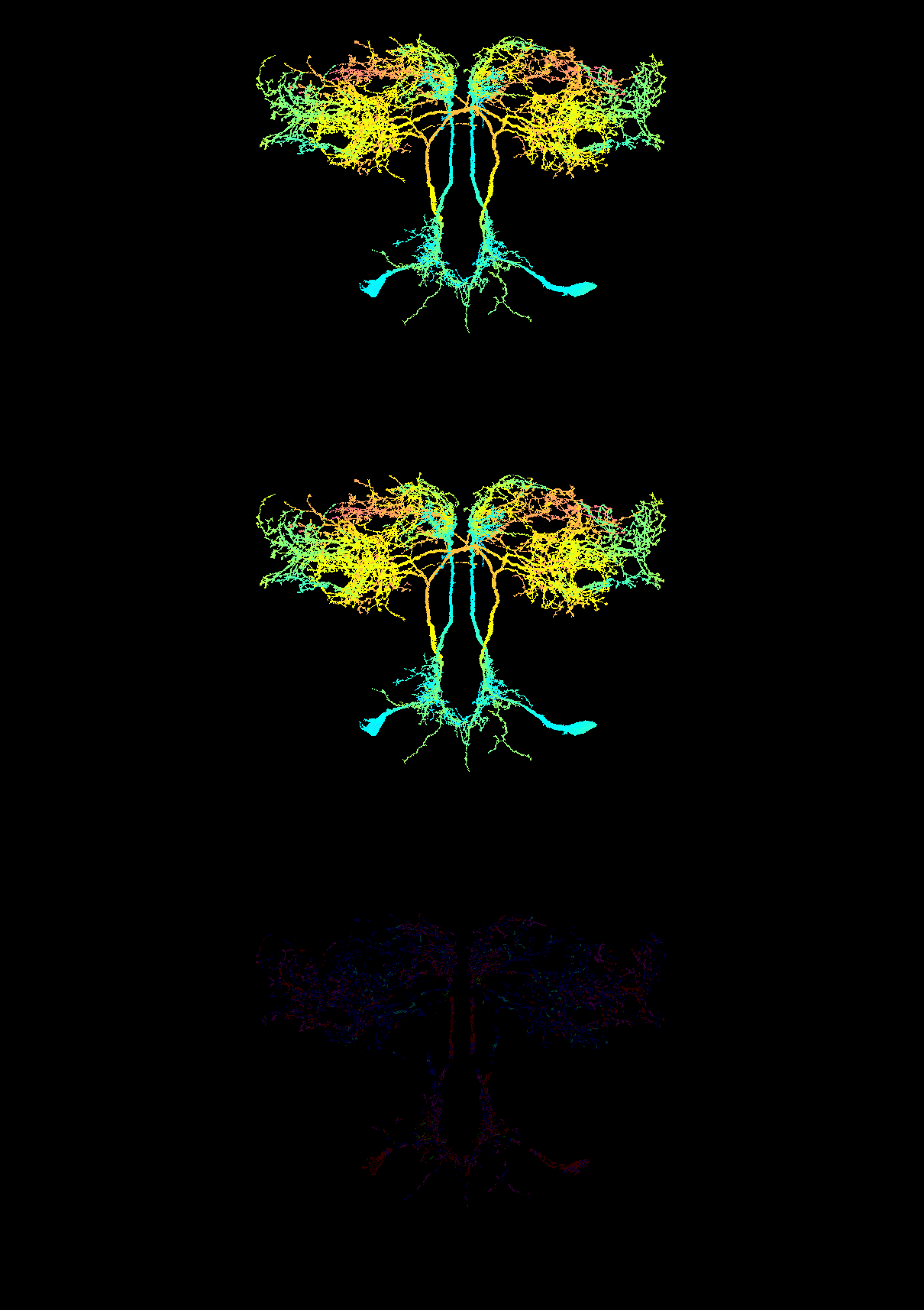
The bilateral SEZ AstA pair is unambiguous — anterior somas in
cyan/teal, arbours sweeping dorsally into the SMP/SLP through yellow →
orange → red. Both back-ends agree on 2,033,613 / 2,054,580
pixels (98.98%) exactly; the remainder differ by at
most 1/255 RGB unit (the skimage HSV-roundtrip artefact
mentioned above). The reproducer is
inst/scripts/colormip_methods_panel.R, which uses the
cached sub-sampled point cloud at
inst/extdata/asta1/banc_asta1_points_nm.rds so it runs
without fetching the 50 MB draco meshes.
The algorithm in three lines
zmax <- apply(vol, c(1, 2), which.max)              # 1..nz, first occurrence
maxv <- apply(vol, c(1, 2), max)                    # 0 = background
idx  <- as.integer((zmax - 1) / (dim(vol)[3] - 1) * 255) + 1L
rgb  <- neuronbridger:::colormip_depth_lut[idx, ]   # 256 x 3 LUT
rgb[!maxv > 0, ] <- 0                               # mask background
nrrd_to_mip(method = "direct") adds:
- the
(nx, ny)→(ny, nx)transpose that PNG/TIFF writers expect; - a 90-pixel black header for VNC space, matching the convention that every Janelia VNC colour-MIP carries;
- file/folder dispatch and round-trip writing of PNG / TIFF.
Provenance
- Algorithm: Otsuna et al. 2018, bioRxiv; ColorMIP Mask Search and ColorDepthMIP Generator FIJI plugins (JaneliaSciComp/ColorMIP_Mask_Search).
-
Python port: Stephan Gerhard (braincircuits.io),
shipped as
make_colormip()infanc.render_neuronsinside the BANC fly-connectome package (PyPI:banc). The 256-entry depth LUT used bynrrd_to_mip(method = "direct")is copied verbatim from that file;method = "python"calls the samedepth_lutviareticulate. -
R port: this package; see
R/colormip.Rand the unit tests intests/testthat/test-colormip.Rfor the BANC equivalence check. -
Bridging conventions: lifted from
wilson-lab/nat-tech(hemibrain_to_nrrd,flywireid_to_nrrd).