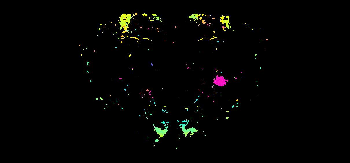
Colour-depth MIPs from a registered LM volume (Kondo 2020 CapaR) in JRC2018U_HR
Source:vignettes/colormip_lm.Rmd
colormip_lm.RmdGoal
Take a registered light-microscopy image volume — here the
Capability receptor staining
IS2_CapaR_no1_02_warp_m0g40c4e1e-1x16r3.nrrd from Kondo et al. 2020,
warped into IS2 template space at 0.41 × 0.41 × 1.07 µm — bridge it into
JRC2018U_HR (the NeuronBridge brain space:
1210 × 566 × 174 voxels at
0.5189 × 0.5189 × 1.0 µm), and render a colour-depth MIP
via nrrd_to_mip(). The output is directly comparable to the
connectome MIPs from the connectome → MIP vignette: same
algorithm, same colour LUT, same grid.
For serving the bridged volume as a Neuroglancer layer alongside BANC (the natural follow-on once you have a JRC2018U-space NRRD in hand), see the LM → Neuroglancer vignette.
Why thresholding matters for LM data
nrrd_to_mip() encodes the most-anterior occupied z-slice
at each (x, y) as a colour. On a binary skeleton or mesh
rendering this just outlines the neuron. On a real confocal stack
every voxel has some signal — autofluorescence, off-target rind
staining, mounting artefacts — so a naive > 0 mask
paints the entire brain volume rainbow.
nrrd_to_mip()’s defaults handle this for you:
-
threshold = "auto"applies Triangle thresholding (Zack et al. 1977) on grayscale input — the same algorithm Janelia’s FIJI macro reaches for as its auto fallback. -
denoise = "auto"applies a3 × 3 × 3median filter to suppress salt-and-pepper noise before the MIP step (the equivalent of FIJI’s Mask Median Subtraction).
Both are skipped for binary input (e.g. the synthetic neuron
voxelisations of the connectome MIP vignette). For power users there are
explicit "otsu", raw-cutoff, and quantile options.
Setup
remotes::install_github("natverse/neuronbridger")
remotes::install_github("natverse/nat.flybrains")    # IS2, JFRC2 templates + CMTK regs
remotes::install_github("natverse/nat.jrcbrains")    # JFRC2 -> JRC2018F -> JRC2018U H5 transforms
nat.jrcbrains::download_saalfeldlab_registrations()  # ~ a few GB; one-time

install.packages("mmand")                            # 3-D median filter (Suggests)
# CMTK: pre-built MacOSX zip from https://www.nitrc.org/projects/cmtk/
# (reformatx is what nat::xformimage shells out to)Where to get the source data
The Kondo et al. 2020 receptor-tagging stacks are hosted on
G-Node: doi.gin.g-node.org/10.12751/g-node.10246f.
Pull the IS2-aligned NRRD for whichever receptor / peptide you want; the
example below uses
IS2_CapaR_no1_02_warp_m0g40c4e1e-1x16r3.nrrd (the
Capability receptor, brain #1, signal channel #2).
Replace NRRD_IN below with the path to your
downloaded copy — the pipeline is identical for any IS2-space
NRRD.
If you cite this data downstream, the canonical reference is:
Kondo, S., Takahashi, T., Yamagata, N., Imanishi, Y., Katow, H., Hiramatsu, S., Lynn, K., Abe, A., Kumaraswamy, A., Tanimoto, H. (2020). Neurochemical organization of the Drosophila brain visualized by endogenously tagged neurotransmitter receptors. Cell Rep. 30(1):284–297.e5. PMID 31914394.
Step 1 — Bridge IS2 → JRC2018U_HR (points pipeline)
The IS2 → JRC2018U bridging chain is
IS2 → FCWB → JRC2018F → JRC2018U: the first hop is CMTK
(ships in nat.flybrains), the next two are H5 transforms
(ship in nat.jrcbrains).
nat.h5reg (the helper that handles H5 transforms)
currently exposes points-mode warping but not
image-mode warping, so the cleanest path for a colour-depth MIP is to do
the bridging on a thresholded point cloud rather than
on the raw image volume:
- Threshold + denoise the IS2 stack (the same
nrrd_to_mip()defaults we’d use anyway). - Take every above-threshold voxel centre as a 3-D point in IS2 microns.
- Transform those points through
IS2 → JRC2018Uvianat.templatebrains::xform_brain()(which dispatches CMTK then H5 per hop). - Voxelise the transformed points into the NeuronBridge
JRC2018U_HRgrid.
For the colour-MIP this is loss-free in the dimensions that matter: the LUT is a function of z-depth alone, so retaining only voxel positions (binary mask) and discarding raw intensities is fine.
suppressMessages({
  library(nat); library(nat.flybrains); library(nat.templatebrains)
  library(nat.jrcbrains); library(neuronbridger); library(mmand)
})
nat.jrcbrains::register_saalfeldlab_registrations()

# Replace with your local path after downloading from G-Node:
#   https://doi.gin.g-node.org/10.12751/g-node.10246f/
NRRD_IN <- "IS2_CapaR_no1_02_warp_m0g40c4e1e-1x16r3.nrrd"

v <- nat::read.nrrd(NRRD_IN)
voxdims_um <- diag(attr(v, "header")[["space directions"]])

# 16-bit -> 8-bit (Kondo stacks have most signal in the bottom 12 bits)
vol <- as.integer(pmin(pmax(as.integer(v), 0L), 4095L) / 16L)
dim(vol) <- dim(v)

# Same auto pipeline as nrrd_to_mip(): 3x3x3 median + Triangle threshold
vol_med <- mmand::medianFilter(vol, mmand::shapeKernel(c(3, 3, 3), type = "box"))
thr <- neuronbridger:::colormip_triangle_threshold(vol_med)

# Foreground voxel centres -> physical microns in IS2 space
fg_idx     <- which(vol_med > thr, arr.ind = TRUE)
pts_is2_um <- sweep(fg_idx - 1L, 2, voxdims_um, "*")

# Transform IS2 -> JRC2018U via the bridging graph (CMTK + H5)
pts_jrc_um <- nat.templatebrains::xform_brain(pts_is2_um,
                                              sample    = "IS2",
                                              reference = "JRC2018U")

# Voxelise into the NeuronBridge JRC2018U_HR grid
JRC2018U_HR <- nat.templatebrains::templatebrain(
  "JRC2018U_HR",
  dims    = c(1210L, 566L, 174L),
  voxdims = c(0.5189, 0.5189, 1.0),
  units   = "microns")
v_jrc <- nat::as.im3d(pts_jrc_um, JRC2018U_HR)
storage.mode(v_jrc) <- "integer"

# Optional: nat::write.nrrd(v_jrc, "CapaR_in_JRC2018U_HR.nrrd")
If a future
nat.h5regadds anxformimagemethod, the entire threshold + voxelise chain above can collapse to a singlexform_brain(v_is2, sample = "IS2", reference = "JRC2018U")call on the original image volume, andnrrd_to_mip()will threshold + denoise the result as it does today. Until then the points pipeline is the practical path through the H5 transforms.
VNC neurons / VNC LM data would replace
reference = "JRC2018U"withreference = "JRCVNC2018U", andtarget_space = "VNC"in Step 2. The current Kondo 2020 collection is brain-only.
Step 2 — Colour-depth MIP
mip_path <- nrrd_to_mip(
  v_jrc,
  savefolder   = "~/lm_mips",
  method       = "direct",
  target_space = "brain"
  # threshold/denoise are auto: they detect that v_jrc is now a binary
  # mask (we already thresholded in Step 1) and skip both. If you skip
  # the points pipeline above and pass a raw grayscale NRRD instead,
  # the defaults run Triangle + 3x3x3 median for you.
)
mip_path
#> "~/lm_mips/colormip.png"
For finer control:
# Stricter: top 1% of foreground signal only (good for sparse cell-body stains)
nrrd_to_mip(v_jrc, threshold = 0.99, denoise = "median3d")

# Otsu rather than Triangle (works better on bimodal foregrounds):
nrrd_to_mip(v_jrc, threshold = "otsu")

# Raw cutoff in source-data units (skip percentile interpretation):
nrrd_to_mip(v_jrc, threshold = 750L)

# Skip thresholding entirely (legacy >0 mask -- only sensible on binary input):
nrrd_to_mip(v_jrc, threshold = "none", denoise = "none")
The same arguments work in method = "python" (calls
Stephan Gerhard’s BANC port via reticulate) and the
back-ends produce byte-equivalent output (sub-1/255 RGB rounding from
skimage’s HSV roundtrip is the only difference).
Validate the back-ends agree
nrrd_to_mip() exposes three interchangeable algorithms
targeting the same Janelia ColorMIP / Color Depth MIP specification
(Otsuna et al. 2018, bioRxiv):
method = |
Implementation | When to use |
|---|---|---|
"direct" (default)
|
Pure R; vectorised which.max + LUT lookup |
The fast path; no JVM, no Python |
"python" |
Stephan
Gerhard’s BANC port called via reticulate
|
Validate against the upstream Python implementation |
"fiji" |
Janelia’s Color_Depth_MIP_batch_0308_2021.ijm
macro |
Run the canonical FIJI implementation if you already have it installed |
Apply the same threshold + denoise (so the comparison is apples-to-apples) and check pixel agreement:
mip_r  <- nrrd_to_mip(v_jrc, save = FALSE, method = "direct",  target_space = "brain")
mip_py <- nrrd_to_mip(v_jrc, save = FALSE, method = "python", target_space = "brain")

max_diff <- max(abs(mip_r - mip_py))
sprintf("Max abs diff R vs Python: %.4f  (%d / 255 RGB units)",
        max_diff, as.integer(round(max_diff * 255)))
sprintf("Pixels exactly equal: %d / %d (%.4f%%)",
        sum(mip_r == mip_py), length(mip_r),
        100 * sum(mip_r == mip_py) / length(mip_r))
Typical numbers on the BANC AstA1 connectome MIP (synthetic neuron
voxelisation): 2 049 816 / 2 054 580 pixels exactly equal
(99.77%), the rest off by exactly 1/255 — the rounding artefact
from skimage’s rgb2hsv → hsv2rgb roundtrip in the BANC
code; the R back-end skips that roundtrip because every depth-LUT entry
already has maximum brightness, making it mathematically a no-op.
method = "fiji" reproduces this validation against the
original Janelia macro; it requires a working FIJI install with the
ColorMIP plugins from JaneliaSciComp/ColorMIP_Mask_Search.
Self-contained sanity check (no IS2, no transforms)
The chunk below builds a tiny synthetic noisy 3-D volume — a single bright “cell body” buried in Gaussian noise — and checks that the default threshold + denoise carve it out cleanly.
library(neuronbridger)

set.seed(3)
vol <- array(as.integer(pmin(pmax(rnorm(40 * 40 * 30, 15, 4), 0), 255)),
             dim = c(40L, 40L, 30L))
vol[18:22, 18:22, 14:16] <- 200L

mip_default <- nrrd_to_mip(vol, save = FALSE, method = "direct",
                           target_space = "brain")
mip_naive   <- nrrd_to_mip(vol, save = FALSE, method = "direct",
                           target_space = "brain",
                           threshold = "none", denoise = "none")

# Naive: every noisy voxel becomes foreground.
# Default: only the bright blob does.
fg_default <- mean(apply(mip_default, c(1, 2), max) > 0)
fg_naive   <- mean(apply(mip_naive,   c(1, 2), max) > 0)
sprintf("naive %.1f%% fg vs default %.1f%% fg", 100 * fg_naive, 100 * fg_default)
#> [1] "naive 100.0% fg vs default 1.8% fg"
Provenance
- Source data: Kondo, S. et al. (2020). Neurochemical organization of the Drosophila brain visualized by endogenously tagged neurotransmitter receptors. Cell Rep. 30(1):284-297.e5.
- MIP algorithm: Otsuna et al. 2018, bioRxiv; thresholding via Zack et al. 1977 (Triangle); denoising via a 3-D median filter, the equivalent of the FIJI plugin’s Mask Median Subtraction step.
-
Bridging conventions: lifted from
wilson-lab/nat-tech. -
JRC2018U_HR grid: 1210 × 566 × 174 at 0.5189 ×
0.5189 × 1.0 µm, the NeuronBridge brain space
(
JRC2018_UNISEX_20x_HRin BANC’stemplate_spaces).