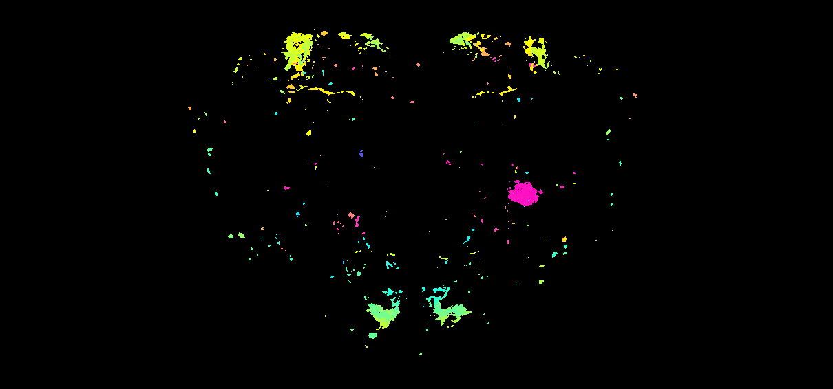
Goal
Take a registered light-microscopy volume — here the
Capability receptor staining
IS2_CapaR_no1_02_warp_m0g40c4e1e-1x16r3.nrrd from Kondo et al. 2020,
warped into IS2 at 0.41 × 0.41 × 1.07 µm — bridge it into
JRC2018U_HR (NeuronBridge brain space,
1210 × 566 × 174 voxels at
0.5189 × 0.5189 × 1.0 µm), and render a colour-depth MIP
via nrrd_to_mip(). The output is directly comparable to the
connectome MIPs from Render a MIP from an
EM neuron — same algorithm, same colour LUT, same grid.
To serve the bridged volume as a Neuroglancer layer alongside BANC, see Publish an LM volume as a Neuroglancer layer on BANC.
Why thresholding matters for LM data
nrrd_to_mip() encodes the most-anterior occupied z-slice
at each (x, y) as a colour. On a binary skeleton or mesh
rendering this just outlines the neuron. On a real confocal stack
every voxel has some signal — autofluorescence, off-target rind
staining, mounting artefacts — so a naive > 0 mask
paints the entire brain volume rainbow.
nrrd_to_mip()’s defaults handle this for you:
-
threshold = "auto"applies Triangle thresholding (Zack et al. 1977) on grayscale input — the same algorithm Janelia’s FIJI macro reaches for as its auto fallback. -
denoise = "auto"applies a3 × 3 × 3median filter to suppress salt-and-pepper noise before the MIP step (the equivalent of FIJI’s Mask Median Subtraction).
Both are skipped for binary input (e.g. the synthetic neuron
voxelisations of the EM-MIP vignette).
For power users there are explicit "otsu", raw-cutoff, and
quantile options.
Setup
remotes::install_github("natverse/neuronbridger")
remotes::install_github("natverse/nat.flybrains")    # IS2, JFRC2 templates + CMTK regs
remotes::install_github("natverse/nat.jrcbrains")    # JFRC2 -> JRC2018F -> JRC2018U H5 transforms
nat.jrcbrains::download_saalfeldlab_registrations()  # ~ a few GB; one-time

install.packages("mmand")                            # 3-D median filter (Suggests)
# CMTK: pre-built MacOSX zip from https://www.nitrc.org/projects/cmtk/
# (reformatx is what nat::xformimage shells out to)Where to get the source data
The Kondo et al. 2020 receptor-tagging stacks are hosted on
G-Node: doi.gin.g-node.org/10.12751/g-node.10246f.
Pull the IS2-aligned NRRD for whichever receptor / peptide you want; the
example below uses
IS2_CapaR_no1_02_warp_m0g40c4e1e-1x16r3.nrrd (the
Capability receptor, brain #1, signal channel #2).
Replace NRRD_IN below with the path to your
downloaded copy — the pipeline is identical for any IS2-space
NRRD.
If you cite this data downstream, the canonical reference is:
Kondo, S., Takahashi, T., Yamagata, N., Imanishi, Y., Katow, H., Hiramatsu, S., Lynn, K., Abe, A., Kumaraswamy, A., Tanimoto, H. (2020). Neurochemical organization of the Drosophila brain visualized by endogenously tagged neurotransmitter receptors. Cell Rep. 30(1):284–297.e5. PMID 31914394.
Step 1 — Bridge IS2 → JRC2018U_HR (points pipeline)
The IS2 → JRC2018U bridging chain is
IS2 → FCWB → JRC2018F → JRC2018U: the first hop is CMTK
(ships in nat.flybrains), the next two are H5 transforms
(ship in nat.jrcbrains).
nat.h5reg (the helper that handles H5 transforms)
currently exposes points-mode warping but not
image-mode warping, so the cleanest path for a colour-depth MIP is to do
the bridging on a thresholded point cloud rather than
on the raw image volume:
- Threshold + denoise the IS2 stack (the same
nrrd_to_mip()defaults we’d use anyway). - Take every above-threshold voxel centre as a 3-D point in IS2 microns.
- Transform those points through
IS2 → JRC2018Uvianat.templatebrains::xform_brain()(which dispatches CMTK then H5 per hop). - Voxelise the transformed points into the NeuronBridge
JRC2018U_HRgrid.
For the colour-MIP this is loss-free in the dimensions that matter: the LUT is a function of z-depth alone, so retaining only voxel positions (binary mask) and discarding raw intensities is fine.
suppressMessages({
  library(nat); library(nat.flybrains); library(nat.templatebrains)
  library(nat.jrcbrains); library(neuronbridger); library(mmand)
})
nat.jrcbrains::register_saalfeldlab_registrations()

# Replace with your local path after downloading from G-Node:
#   https://doi.gin.g-node.org/10.12751/g-node.10246f/
NRRD_IN <- "IS2_CapaR_no1_02_warp_m0g40c4e1e-1x16r3.nrrd"

v <- nat::read.nrrd(NRRD_IN)
voxdims_um <- diag(attr(v, "header")[["space directions"]])

# 16-bit -> 8-bit (Kondo stacks have most signal in the bottom 12 bits)
vol <- as.integer(pmin(pmax(as.integer(v), 0L), 4095L) / 16L)
dim(vol) <- dim(v)

# Same auto pipeline as nrrd_to_mip(): 3x3x3 median + Triangle threshold
vol_med <- mmand::medianFilter(vol, mmand::shapeKernel(c(3, 3, 3), type = "box"))
thr <- neuronbridger:::colormip_triangle_threshold(vol_med)

# Foreground voxel centres -> physical microns in IS2 space
fg_idx     <- which(vol_med > thr, arr.ind = TRUE)
pts_is2_um <- sweep(fg_idx - 1L, 2, voxdims_um, "*")

# Transform IS2 -> JRC2018U via the bridging graph (CMTK + H5)
pts_jrc_um <- nat.templatebrains::xform_brain(pts_is2_um,
                                              sample    = "IS2",
                                              reference = "JRC2018U")

# Voxelise into the NeuronBridge JRC2018U_HR grid
JRC2018U_HR <- nat.templatebrains::templatebrain(
  "JRC2018U_HR",
  dims    = c(1210L, 566L, 174L),
  voxdims = c(0.5189, 0.5189, 1.0),
  units   = "microns")
v_jrc <- nat::as.im3d(pts_jrc_um, JRC2018U_HR)
storage.mode(v_jrc) <- "integer"

# Optional: nat::write.nrrd(v_jrc, "CapaR_in_JRC2018U_HR.nrrd")
If a future
nat.h5regadds anxformimagemethod, the entire threshold + voxelise chain above can collapse to a singlexform_brain(v_is2, sample = "IS2", reference = "JRC2018U")call on the original image volume, andnrrd_to_mip()will threshold + denoise the result as it does today. Until then the points pipeline is the practical path through the H5 transforms.
VNC neurons / VNC LM data would replace
reference = "JRC2018U"withreference = "JRCVNC2018U", andtarget_space = "VNC"in Step 2. The current Kondo 2020 collection is brain-only.
Step 2 — Colour-depth MIP
mip_path <- nrrd_to_mip(
  v_jrc,
  savefolder   = "~/lm_mips",
  method       = "direct",
  target_space = "brain"
  # threshold/denoise are auto: they detect that v_jrc is now a binary
  # mask (we already thresholded in Step 1) and skip both. If you skip
  # the points pipeline above and pass a raw grayscale NRRD instead,
  # the defaults run Triangle + 3x3x3 median for you.
)
mip_path
#> "~/lm_mips/colormip.png"
For finer control:
# Stricter: top 1% of foreground signal only (good for sparse cell-body stains)
nrrd_to_mip(v_jrc, threshold = 0.99, denoise = "median3d")

# Otsu rather than Triangle (works better on bimodal foregrounds):
nrrd_to_mip(v_jrc, threshold = "otsu")

# Raw cutoff in source-data units (skip percentile interpretation):
nrrd_to_mip(v_jrc, threshold = 750L)

# Skip thresholding entirely (legacy >0 mask -- only sensible on binary input):
nrrd_to_mip(v_jrc, threshold = "none", denoise = "none")
The same arguments work in method = "python" (calls
Jasper Phelps’s BANC port via reticulate) and the back-ends
produce byte-equivalent output (sub-1/255 RGB rounding from skimage’s
HSV roundtrip is the only difference).
Validate the back-ends agree
nrrd_to_mip() exposes three interchangeable algorithms
targeting the same Janelia ColorMIP / Color Depth MIP specification
(Otsuna et al. 2018, bioRxiv):
method = |
Implementation | When to use |
|---|---|---|
"direct" (default)
|
Pure R; vectorised which.max + LUT lookup |
The fast path; no JVM, no Python |
"python" |
Jasper
Phelps’s BANC port called via reticulate
|
Validate against the upstream Python implementation |
"fiji" |
Janelia’s Color_Depth_MIP_batch_0308_2021.ijm
macro |
Run the canonical FIJI implementation if you already have it installed |
Apply the same threshold + denoise (so the comparison is apples-to-apples) and check pixel agreement:
mip_r  <- nrrd_to_mip(v_jrc, save = FALSE, method = "direct",  target_space = "brain")
mip_py <- nrrd_to_mip(v_jrc, save = FALSE, method = "python", target_space = "brain")

max_diff <- max(abs(mip_r - mip_py))
sprintf("Max abs diff R vs Python: %.4f  (%d / 255 RGB units)",
        max_diff, as.integer(round(max_diff * 255)))
sprintf("Pixels exactly equal: %d / %d (%.4f%%)",
        sum(mip_r == mip_py), length(mip_r),
        100 * sum(mip_r == mip_py) / length(mip_r))
Typical numbers on the BANC AstA1 connectome MIP (synthetic neuron
voxelisation): 2 049 816 / 2 054 580 pixels exactly equal
(99.77%), the rest off by exactly 1/255 — the rounding artefact
from skimage’s rgb2hsv → hsv2rgb roundtrip in the BANC
code; the R back-end skips that roundtrip because every depth-LUT entry
already has maximum brightness, making it mathematically a no-op.
method = "fiji" reproduces this validation against the
original Janelia macro; it requires a working FIJI install with the
ColorMIP plugins from JaneliaSciComp/ColorMIP_Mask_Search.
Self-contained sanity check (no IS2, no transforms)
The chunk below builds a tiny synthetic noisy 3-D volume — a single bright “cell body” buried in Gaussian noise — and checks that the default threshold + denoise carve it out cleanly.
library(neuronbridger)

set.seed(3)
vol <- array(as.integer(pmin(pmax(rnorm(40 * 40 * 30, 15, 4), 0), 255)),
             dim = c(40L, 40L, 30L))
vol[18:22, 18:22, 14:16] <- 200L

mip_default <- nrrd_to_mip(vol, save = FALSE, method = "direct",
                           target_space = "brain")
mip_naive   <- nrrd_to_mip(vol, save = FALSE, method = "direct",
                           target_space = "brain",
                           threshold = "none", denoise = "none")

# Naive: every noisy voxel becomes foreground.
# Default: only the bright blob does.
fg_default <- mean(apply(mip_default, c(1, 2), max) > 0)
fg_naive   <- mean(apply(mip_naive,   c(1, 2), max) > 0)
sprintf("naive %.1f%% fg vs default %.1f%% fg", 100 * fg_naive, 100 * fg_default)
#> [1] "naive 100.0% fg vs default 1.8% fg"
Provenance
- Source data: Kondo, S. et al. (2020). Neurochemical organization of the Drosophila brain visualized by endogenously tagged neurotransmitter receptors. Cell Rep. 30(1):284-297.e5.
- MIP algorithm: Otsuna et al. 2018, bioRxiv; thresholding via Zack et al. 1977 (Triangle); denoising via a 3-D median filter, the equivalent of the FIJI plugin’s Mask Median Subtraction step.
-
Bridging conventions: lifted from
wilson-lab/nat-tech. -
JRC2018U_HR grid: 1210 × 566 × 174 at 0.5189 ×
0.5189 × 1.0 µm, the NeuronBridge brain space
(
JRC2018_UNISEX_20x_HRin BANC’stemplate_spaces).