Intro
In Fig 6 of our manuscript Schlegel et al 2023 we show an example of across-dataset cell typing using AOTU063 as an example.
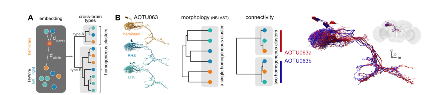
We should be able to recapitulate the basic features of this analysis here.
For this analysis we will use the version 630 connectivity / annotation data released in June 2023. We will set an option use the lower level fafbseg package to ensure this. You may need to download the relevant data dumps if you have not done so previously.
fafbseg::download_flywire_release_data(version = 630)
#> Checking for connectivity files to download
#> Checking for annotation files to download
#> Loading required namespace: git2r
fafbseg::flywire_connectome_data_version(set = 630)
aotu63=cf_meta(cf_ids(query = '/type:AOTU063.*', datasets = c("flywire","hemibrain")))
aotu63
#>                   id side   class subclass subsubclass     type
#> 1 720575940620326253    R central     <NA>        <NA> AOTU063a
#> 2 720575940618697118    L central     <NA>        <NA> AOTU063b
#> 3 720575940621925631    R central     <NA>        <NA> AOTU063b
#> 4 720575940631129362    L central     <NA>        <NA> AOTU063a
#> 5          791039731    R    <NA>     <NA>        <NA>  AOTU063
#> 6          800929667    R    <NA>     <NA>        <NA>  AOTU063
#>            lineage group tissue sex          instance   dataset
#> 1 putative_primary  <NA>  brain   F        AOTU063a_R   flywire
#> 2 putative_primary  <NA>  brain   F        AOTU063b_L   flywire
#> 3 putative_primary  <NA>  brain   F        AOTU063b_R   flywire
#> 4 putative_primary  <NA>  brain   F        AOTU063a_L   flywire
#> 5             <NA>  <NA>  brain   F AOTU063(SCB058)_R hemibrain
#> 6             <NA>  <NA>  brain   F AOTU063(SCB058)_R hemibrain
#>                     key
#> 1 fw:720575940620326253
#> 2 fw:720575940618697118
#> 3 fw:720575940621925631
#> 4 fw:720575940631129362
#> 5          hb:791039731
#> 6          hb:800929667
aotu63 %>%
  cf_cosine_plot()
#> Matching types across datasets. Keeping 320/445 output connections with total weight 8726/11012 (79%)
#> Matching types across datasets. Keeping 720/1082 input connections with total weight 13850/18107 (76%)
#> Warning in coconat::partner_summary2adjacency_matrix(x[["outputs"]], inputcol =
#> "pre_key", : Dropping: 73/320 neurons representing 955/8726 synapses due to
#> missing ids!
#> Warning in coconat::partner_summary2adjacency_matrix(x[["inputs"]], inputcol =
#> groupcol, : Dropping: 60/720 neurons representing 778/13850 synapses due to
#> missing ids!
We can get the dendrogram for this clustering
aotu63.hc = cf_cosine_plot(aotu63, heatmap = FALSE)
#> Matching types across datasets. Keeping 320/445 output connections with total weight 8726/11012 (79%)
#> Matching types across datasets. Keeping 720/1082 input connections with total weight 13850/18107 (76%)
#> Warning in coconat::partner_summary2adjacency_matrix(x[["outputs"]], inputcol =
#> "pre_key", : Dropping: 73/320 neurons representing 955/8726 synapses due to
#> missing ids!
#> Warning in coconat::partner_summary2adjacency_matrix(x[["inputs"]], inputcol =
#> groupcol, : Dropping: 60/720 neurons representing 778/13850 synapses due to
#> missing ids!
plot(aotu63.hc)
And then cut it in two and extract those two clusters using the
coconat::add_cluster_info() helper function.
aotu63=coconat::add_cluster_info(aotu63, dend=aotu63.hc, k=2)
#> Warning in coconat::add_cluster_info(aotu63, dend = aotu63.hc, k = 2): Multiple standard id columns are present in aotu63
#> Choosing key
aotu63 %>%
  select(side, type, dataset, group_k2, key) %>%
  arrange(group_k2, side)
#>   side     type   dataset group_k2                   key
#> 1    L AOTU063a   flywire        1 fw:720575940631129362
#> 2    R AOTU063a   flywire        1 fw:720575940620326253
#> 3    R  AOTU063 hemibrain        1          hb:800929667
#> 4    L AOTU063b   flywire        2 fw:720575940618697118
#> 5    R AOTU063b   flywire        2 fw:720575940621925631
#> 6    R  AOTU063 hemibrain        2          hb:791039731
So from this we can see that group 2 seems to the “b” type.
Finding the partners that define the types
What might distinguish these two types? We can fetch, say, the input partners, and then look at how connection strength varies across the types.
To get started let’s redefine the type of our 6 query neurons based
on the clustering. Then fetch the input partners and merge in the the
AOTU063 type (i.e. AOTU063a or AOTU063b) as a new column called
qtype
aotu63v2=aotu63 %>%
  mutate(type=case_when(
    group_k2==1 ~ 'AOTU063a',
    group_k2==2 ~ 'AOTU063b'
  ))
aotu63in <- cf_partners(aotu63, partners = 'in', threshold = 10)
aotu63in
#> # A tibble: 657 × 16
#>     pre_id post_id weight dataset tissue sex   pre_key      post_key side  class
#>    <int64> <int64>  <int> <chr>   <chr>  <chr> <chr>        <chr>    <chr> <chr>
#>  1    7e17    7e17    118 flywire brain  F     fw:72057594… fw:7205… R     visu…
#>  2    7e17    7e17    109 flywire brain  F     fw:72057594… fw:7205… R     visu…
#>  3    7e17    7e17    109 flywire brain  F     fw:72057594… fw:7205… R     cent…
#>  4    7e17    7e17     96 flywire brain  F     fw:72057594… fw:7205… L     visu…
#>  5    7e17    7e17     95 flywire brain  F     fw:72057594… fw:7205… R     visu…
#>  6    7e17    7e17     90 flywire brain  F     fw:72057594… fw:7205… L     cent…
#>  7    7e17    7e17     87 flywire brain  F     fw:72057594… fw:7205… R     cent…
#>  8    7e17    7e17     83 flywire brain  F     fw:72057594… fw:7205… R     visu…
#>  9    7e17    7e17     83 flywire brain  F     fw:72057594… fw:7205… R     cent…
#> 10    7e17    7e17     82 flywire brain  F     fw:72057594… fw:7205… R     cent…
#> # ℹ 647 more rows
#> # ℹ 6 more variables: subclass <chr>, subsubclass <chr>, type <chr>,
#> #   lineage <chr>, group <chr>, instance <chr>
# note that AOTU063 neurons will be the postsynaptic partners in this dataframe
aotu63in <- aotu63in %>%
  left_join(
    aotu63v2 %>% mutate(qtype=type) %>% select(qtype, key),
    by=c("post_key"='key'))
aotu63in %>%
  select(weight, type, qtype)
#> # A tibble: 657 × 3
#>    weight type    qtype
#>     <int> <chr>   <chr>
#>  1    118 LT52    AOTU063b
#>  2    109 LT52    AOTU063b
#>  3    109 AOTU041 AOTU063a
#>  4     96 LT52    AOTU063b
#>  5     95 LT52    AOTU063b
#>  6     90 AOTU042 AOTU063a
#>  7     87 SIP034  AOTU063a
#>  8     83 LT52    AOTU063b
#>  9     83 AOTU041 AOTU063a
#> 10     82 AOTU014 AOTU063b
#> # ℹ 647 more rows
Ok with that preparatory work we can now make a summary of the inputs across the different types and datasets. This pipeline is a little more involved, but I have commented extensively and if you follow step by step it does make sense.
aotu63in %>%
  mutate(dataset=abbreviate_datasets(dataset)) %>%
  # FlyWire has e.g. LC10a LC10c annotated, but not hemibrain
  mutate(type=case_when(
    grepl("LC10", type) ~ "LC10",
    T ~ type
  )) %>%
  # summarise the connection strength by query cell type, data set
  # and partner (downstream) cell type
  group_by(qtype, dataset, type) %>%
  summarise(weight=sum(weight)) %>%
  # sort with strongest partners first
  arrange(desc(weight)) %>%
  # make four columns, one for each query type / dataset combination
  tidyr::pivot_wider(
    names_from = c(qtype, dataset),
    values_from = weight,
    values_fill = 0) %>%
  # convert from synaptic counts to percentages of total input
  mutate(across(-type, ~round(100*.x/sum(.x))))
#> `summarise()` has regrouped the output.
#> ℹ Summaries were computed grouped by qtype, dataset, and type.
#> ℹ Output is grouped by qtype and dataset.
#> ℹ Use `summarise(.groups = "drop_last")` to silence this message.
#> ℹ Use `summarise(.by = c(qtype, dataset, type))` for per-operation grouping
#>   (`?dplyr::dplyr_by`) instead.
#> # A tibble: 43 × 5
#>    type    AOTU063a_fw AOTU063b_fw AOTU063a_hb AOTU063b_hb
#>    <chr>         <dbl>       <dbl>       <dbl>       <dbl>
#>  1 LC10             56          48          56          45
#>  2 LT52              7          30          11          26
#>  3 SIP034            7           0           5           0
#>  4 NA                6           3           1           6
#>  5 AOTU041           5           2           5           1
#>  6 AOTU042           4           3           3           2
#>  7 AOTU014           0           5           0           5
#>  8 VES041            3           0           3           0
#>  9 AOTU065           2           1           2           2
#> 10 AOTU028           2           0           2           0
#> # ℹ 33 more rows
So we can see that the top few cell types already suggest a number of likely explanations.
For example LC10 provides 10% more input for AOTU063a vs AOTU063b while LT52 input is much stronger for AOTU063b than AOTU063a. Crucially these patterns are consistent across datasets.
Distinctive output partners
aotu63out <- cf_partners(aotu63, partners = 'out', threshold = 10)

aotu63out <- aotu63out %>%
  left_join(
    aotu63v2 %>% mutate(qtype=type) %>% select(qtype, key),
    by=c("pre_key"='key'))

aotu63out %>%
  mutate(dataset=abbreviate_datasets(dataset)) %>%
  # FlyWire has e.g. LC10a LC10c annotated, but not hemibrain
  mutate(type=case_when(
    grepl("LC10", type) ~ "LC10",
    T ~ type
  )) %>%
  group_by(qtype, dataset, type) %>%
  summarise(weight=sum(weight)) %>%
  arrange(desc(weight)) %>%
  tidyr::pivot_wider(names_from = c(qtype, dataset), values_from = weight, values_fill = 0) %>%
  # convert from raw to pct
  mutate(across(-type, ~round(100*.x/sum(.x))))
#> `summarise()` has regrouped the output.
#> ℹ Summaries were computed grouped by qtype, dataset, and type.
#> ℹ Output is grouped by qtype and dataset.
#> ℹ Use `summarise(.groups = "drop_last")` to silence this message.
#> ℹ Use `summarise(.by = c(qtype, dataset, type))` for per-operation grouping
#>   (`?dplyr::dplyr_by`) instead.
#> # A tibble: 57 × 5
#>    type    AOTU063a_fw AOTU063a_hb AOTU063b_fw AOTU063b_hb
#>    <chr>         <dbl>       <dbl>       <dbl>       <dbl>
#>  1 IB008            15          14          11           9
#>  2 NA                5          22           0           7
#>  3 DNa10            12           9          11           7
#>  4 IB010            11           8           5           5
#>  5 AOTU007           8           6           7           8
#>  6 DNde002           3           0           9           0
#>  7 VES064            7           5           4           4
#>  8 DNae011           7           0           3           0
#>  9 DNbe004           6           0           0           0
#> 10 AOTU024           1           1           6           2
#> # ℹ 47 more rows
Here things are not quite obvious but IB008/IB010 look different and some of the newly defined DNs in FlyWire like DNde002/DNbe004/DNae011 look like they might be interesting.