Making surface meshes

Intro

You can use 3D data pulled from CATMAID to create meshes. You can also do the same with light level data and then transform into FAFB space.

Setup

First load main packages

library(elmr)
cl=try(catmaid_login())
catmaid_available=inherits(cl, "catmaid_connection")
library(knitr)
opts_chunk$set(eval=catmaid_available)

In order to run some of this example we need to ensure that we:

can login to the FAFB CATMAID server

We will most our examples run conditionally based on this.

library(dplyr)
library(alphashape3d)
library(rgl)
# set up for 3d plots based on rgl package
rgl::setupKnitr()
# frontal view
view3d(userMatrix=rgl::rotationMatrix(angle = pi, 1,0,0), zoom=0.8)

Selecting synapses

We’re going to use synapses between PNs and KCs to define a mesh. Note that we only use the RHS PNS.

pntokc = catmaid_get_connectors_between(pre_skids = 'WTPN2017_mALT_right',
                                        post_skids = 'KC')
# select 3d position of presynaptic connectors
pntokc %>%
  distinct(connector_id, .keep_all=TRUE) %>%
  select(connector_x:connector_z) %>%
  data.matrix -> cxyz

Where are those points in the brain?

points3d(cxyz, col='red')
plot3d(FAFB)

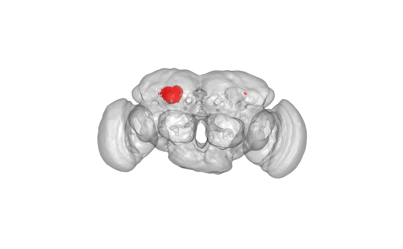
Oh, we still need to remove some points that are distant from the others i.e. on wrong side of brain or too far forward (i.e. not in calyx). They may come from e.g. bilateral PNs making connections on both sides of the brain.

# pick 100 random points
set.seed(42)
s=sample(nrow(cxyz), 100)
sxyz=cxyz[s,]
# knn is normally used for nearest neighbour calculation of a point subset
# but here we do a brute force calculation against all target points
nnres <- nabor::knn(sxyz, cxyz, searchtype = "brute", k=100)
# mean distance from those 100 target points
meand=rowMeans(nnres$nn.dists)
hist(meand, col='red', ylim=c(0,100), br=100)

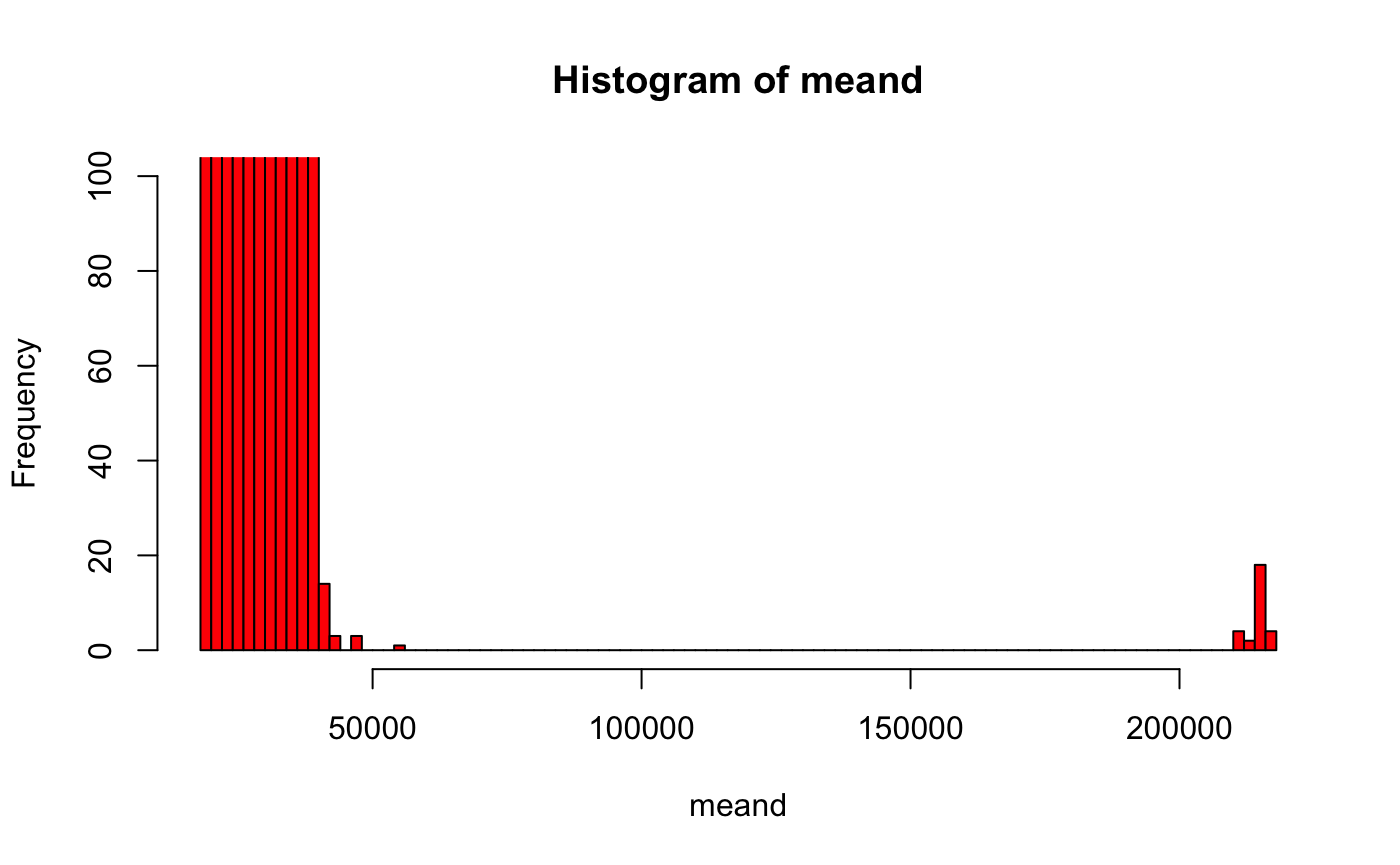
Let’s take everything less than 50,000 nm

cxyz.orig=cxyz
cxyz=cxyz[meand<50e3,]

We could of course use fancier criteria based on dispersion, quantiles etc.

Where are the selected points in the brain?

points3d(cxyz, col='red')
points3d(cxyz.orig, col='black')
plot3d(FAFB)

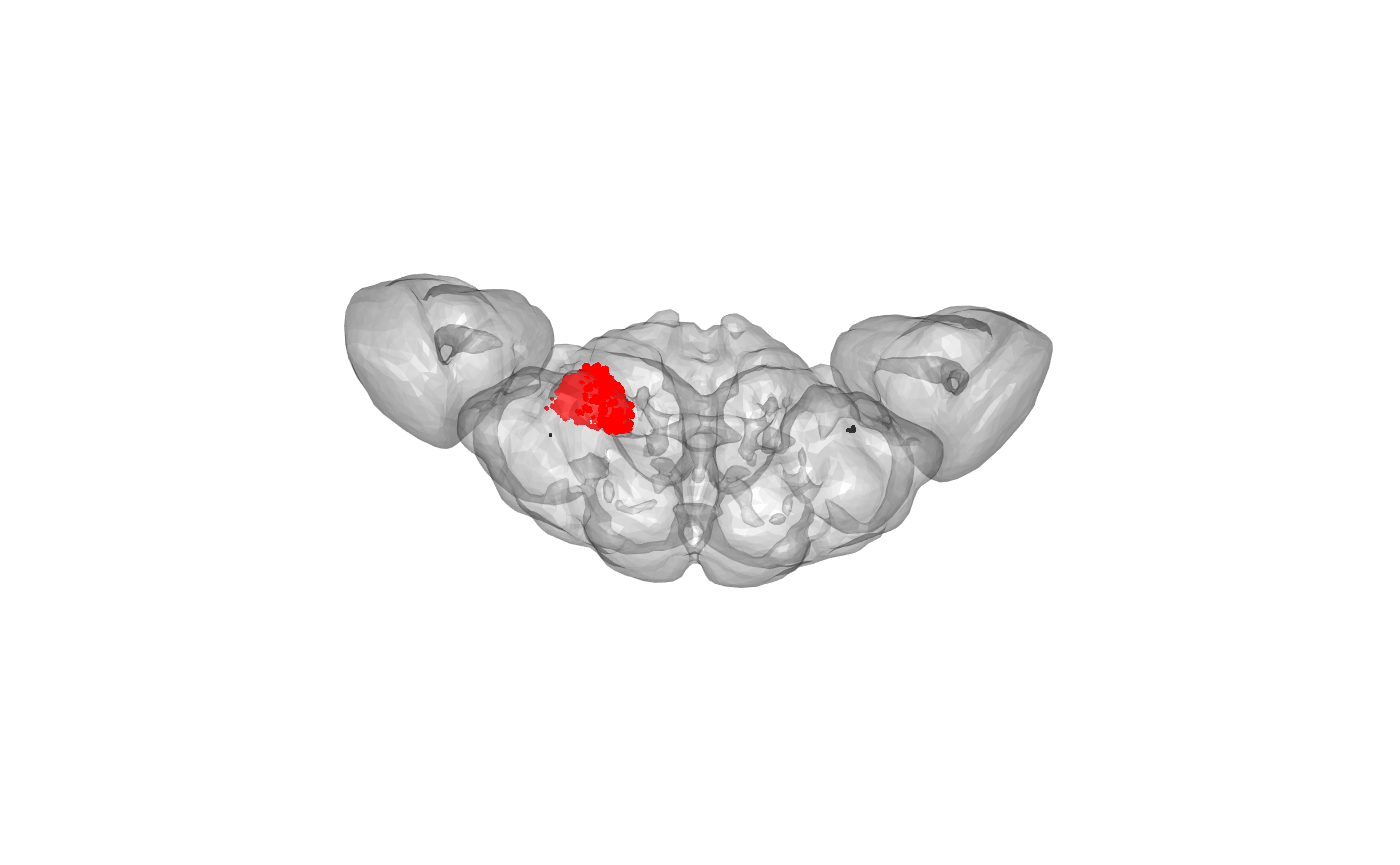
OK, that looks good. Now we can make an alphashape based on those connector positions. We need to set the alpha value in the ashape3d() function to something sensible based on the spatial scale of our data - he we use alpha=6000 nm.

calyx.a=ashape3d(cxyz, alpha = 6000)
calyx=as.mesh3d(calyx.a)

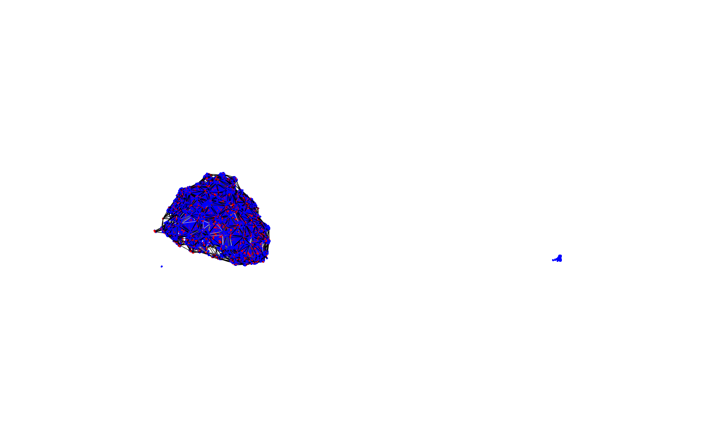
We can compare the resultant mesh with the location of the connectors

wire3d(calyx)
points3d(cxyz, col='red')
points3d(pntokc[,c('post_node_x','post_node_y','post_node_z')], col='blue')

We can also compare with the mesh supplied with elmr, which was transformed from JFRC2 space via JFRC2013 to FAFB:

wire3d(calyx)
plot3d(FAFBNP.surf, "MB_CA_R", alpha=.3)
view3d(userMatrix=rgl::rotationMatrix(angle = pi, 1,0,0), zoom=0.8)

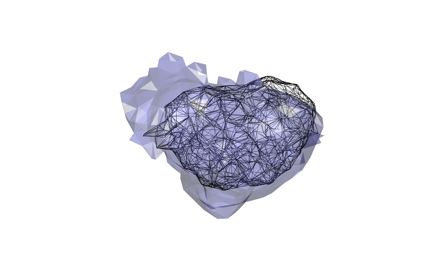
And we can also compare the dorsal view as well:

wire3d(calyx)
plot3d(FAFBNP.surf, "MB_CA_R", alpha=.3)
view3d(userMatrix=rgl::rotationMatrix(angle = -pi/2, 1,0,0), zoom=0.8)

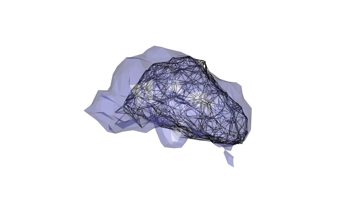
It’s clear that there is a mismatch here. This may originate in part from the fact that the JFRC2013 intermediate template has rather flattened MB calyces. The quality of the JFRC2-JFRC2013 bridging registration is likely also a factor.

Finally if one wanted to place this mesh into CATMAID, one could do it as follows:

catmaid_add_volume(calyx, title="fafb14.pn-kc.MB_CA_R",
                   comment="Constructed by GSXEJ from PN-KC synapses directly in FAFB14 space.")

Gregory Jefferis

2020-06-08

Intro

Setup

Selecting synapses