
coconatfly enables comparative/integrative connectomics across Drosophila datasets. The philosophy is to provide access to the most important functions for connectome analysis in a way that is both convenient and uniform across Drosophila datasets. The package builds upon the coconat package which provides more basic and/or dataset agnostic functionality. In case you were wondering, coconat stands for COmparative COnnectomics for the NATverse and coconatfly enables this specifically for fly datasets.
Although the code is already in active use, especially for comparison of the hemibrain and flywire datasets, it remains experimental. Therefore the interface should not yet been relied upon. In particular, it is quite likely that refactoring will abstract more functionality into coconat as time goes by in order to enable more core functionality to be reused.
Datasets
At present the following datasets are supported (dataset names used in the package in brackets):
- Janelia hemibrain (hemibrain)
- Female Adult Fly Brain - FlyWire connectome (flywire)
- Janelia male Ventral Nerve Cord (manc)
- Wei Lee, John Tuthill and colleagues Female Adult Nerve Cord (fanc)
- Janelia Male CNS (malecns)
- Janelia Male Optic Lobe (part of the malecns) (opticlobe)
- Wei Lee and colleagues Brain and Nerve Cord (banc)
All datasets are either public (hemibrain, manc, malecns, flywire, opticlobe) or access can be requested subject to agreeing to certain terms of use (fanc, banc).
Installation
We recommend installing the latest version of coconatfly from github like so:
install.packages('natmanager')
natmanager::install(pkgs = 'coconatfly')
but you may also choose a specific released version for enhanced reproducibility:
natmanager::install(pkgs = 'coconatfly@v0.2.2')Some of the datasets exposed by coconatfly require authentication for access or are still being annotated in private pre-release.
An example
First let’s load the libraries we need
Two important functions are cf_ids() which allows you to specify a set of neurons from one or more datasets and cf_meta() which fetches information about each neuron including its cell type. For example let’s fetch information about DA1 projection neurons:
cf_meta(cf_ids('DA1_lPN', datasets = 'hemibrain'))
#>           id pre post upstream downstream status    statusLabel     voxels
#> 1 1734350788 621 2084     2084       4903 Traced Roughly traced 1174705998
#> 2 1734350908 725 2317     2317       5846 Traced Roughly traced 1382228240
#> 3 1765040289 702 2398     2398       5521 Traced Roughly traced 1380855164
#> 4 5813039315 691 2263     2263       5577 Traced Roughly traced 1016515847
#> 5  722817260 701 2435     2435       5635 Traced Roughly traced 1104413432
#> 6  754534424 646 2364     2364       5309 Traced Roughly traced 1265805547
#> 7  754538881 623 2320     2320       4867 Traced Roughly traced 1217284590
#>   cropped  instance    type lineage notes  soma side class subclass subsubclass
#> 1   FALSE DA1_lPN_R DA1_lPN   AVM02  <NA>  TRUE    R  <NA>     <NA>        <NA>
#> 2   FALSE DA1_lPN_R DA1_lPN   AVM02  <NA>  TRUE    R  <NA>     <NA>        <NA>
#> 3   FALSE DA1_lPN_R DA1_lPN   AVM02  <NA>  TRUE    R  <NA>     <NA>        <NA>
#> 4   FALSE DA1_lPN_R DA1_lPN   AVM02  <NA> FALSE    R  <NA>     <NA>        <NA>
#> 5   FALSE DA1_lPN_R DA1_lPN   AVM02  <NA> FALSE    R  <NA>     <NA>        <NA>
#> 6   FALSE DA1_lPN_R DA1_lPN   AVM02  <NA>  TRUE    R  <NA>     <NA>        <NA>
#> 7   FALSE DA1_lPN_R DA1_lPN   AVM02  <NA>  TRUE    R  <NA>     <NA>        <NA>
#>   group   dataset           key
#> 1  <NA> hemibrain hb:1734350788
#> 2  <NA> hemibrain hb:1734350908
#> 3  <NA> hemibrain hb:1765040289
#> 4  <NA> hemibrain hb:5813039315
#> 5  <NA> hemibrain  hb:722817260
#> 6  <NA> hemibrain  hb:754534424
#> 7  <NA> hemibrain  hb:754538881
We can also do that for multiple brain datasets
da1meta <- cf_meta(cf_ids('DA1_lPN', datasets = c('hemibrain', 'flywire')))
#> Loading required namespace: git2r
head(da1meta)
#>                   id side   class subclass   subsubclass    type      lineage
#> 1 720575940604407468    R central     ALPN uniglomerular DA1_lPN ALl1_ventral
#> 2 720575940623543881    R central     ALPN uniglomerular DA1_lPN ALl1_ventral
#> 3 720575940637469254    R central     ALPN uniglomerular DA1_lPN ALl1_ventral
#> 4 720575940614309535    L central     ALPN uniglomerular DA1_lPN ALl1_ventral
#> 5 720575940617229632    R central     ALPN uniglomerular DA1_lPN ALl1_ventral
#> 6 720575940619385765    L central     ALPN uniglomerular DA1_lPN ALl1_ventral
#>   group  instance dataset                   key
#> 1  <NA> DA1_lPN_R flywire fw:720575940604407468
#> 2  <NA> DA1_lPN_R flywire fw:720575940623543881
#> 3  <NA> DA1_lPN_R flywire fw:720575940637469254
#> 4  <NA> DA1_lPN_L flywire fw:720575940614309535
#> 5  <NA> DA1_lPN_R flywire fw:720575940617229632
#> 6  <NA> DA1_lPN_L flywire fw:720575940619385765
da1meta %>%
  count(dataset, side)
#>     dataset side n
#> 1   flywire    L 8
#> 2   flywire    R 7
#> 3 hemibrain    R 7
We can also fetch connectivity for these neurons:
da1ds <- da1meta %>%
  cf_partners(threshold = 5, partners = 'output')
head(da1ds)
#> # A tibble: 6 × 8
#>    pre_id post_id weight side  type    dataset pre_key               post_key
#>   <int64> <int64>  <int> <chr> <chr>   <chr>   <chr>                 <chr>
#> 1    7e17    7e17     64 L     DA1_vPN flywire fw:720575940605102694 fw:7205759…
#> 2    7e17    7e17     50 L     CB3356  flywire fw:720575940603231916 fw:7205759…
#> 3    7e17    7e17     49 R     LHAV4a4 flywire fw:720575940604407468 fw:7205759…
#> 4    7e17    7e17     48 R     DA1_vPN flywire fw:720575940623303108 fw:7205759…
#> 5    7e17    7e17     46 L     v2LN30  flywire fw:720575940603231916 fw:7205759…
#> 6    7e17    7e17     42 L     DA1_vPN flywire fw:720575940603231916 fw:7205759…
da1ds %>%
  group_by(type, dataset, side) %>%
  summarise(weight=sum(weight), npre=n_distinct(pre_id), npost=n_distinct(post_id))
#> `summarise()` has grouped output by 'type', 'dataset'. You can override using
#> the `.groups` argument.
#> # A tibble: 381 × 6
#> # Groups:   type, dataset [291]
#>    type            dataset   side  weight  npre npost
#>    <chr>           <chr>     <chr>  <int> <int> <int>
#>  1 AL-AST1         flywire   L         31     5     1
#>  2 AL-AST1         flywire   R         18     3     1
#>  3 AL-AST1         hemibrain R         25     3     1
#>  4 APL             flywire   L         43     7     1
#>  5 APL             flywire   R         70     6     1
#>  6 APL             hemibrain R        113     6     1
#>  7 AVLP010         flywire   L         11     2     1
#>  8 AVLP010         flywire   R          5     1     1
#>  9 AVLP011,AVLP012 flywire   L         11     2     1
#> 10 AVLP011,AVLP012 flywire   R         27     3     1
#> # ℹ 371 more rows
Let’s restrict that to types that are observed in both datasets. We do this by counting how many distinct datasets exist for each type in the results.
da1ds.shared_types.wide <- da1ds %>%
  filter(!(dataset=='hemibrain' & side=='L')) %>% # drop truncated hemibrain LHS
  group_by(type) %>%
  mutate(datasets_type=n_distinct(dataset)) %>%
  filter(datasets_type>1) %>%
  group_by(type, dataset, side) %>%
  summarise(weight=sum(weight)) %>%
  mutate(shortdataset=abbreviate_datasets(dataset)) %>%
  tidyr::pivot_wider(id_cols = type, names_from = c(shortdataset,side),
                     values_from = weight, values_fill = 0)
#> `summarise()` has grouped output by 'type', 'dataset'. You can override using
#> the `.groups` argument.
da1ds.shared_types.wide
#> # A tibble: 44 × 4
#> # Groups:   type [44]
#>    type      fw_L  fw_R  hb_R
#>    <chr>    <int> <int> <int>
#>  1 AL-AST1     31    18    25
#>  2 APL         43    70   113
#>  3 DA1_lPN     50    11    73
#>  4 DA1_vPN    250   254   333
#>  5 DL3_lPN      5     0     9
#>  6 DNb05        6     0     5
#>  7 KCg-m     3290  2575  3030
#>  8 LHAD1d2     72    43    15
#>  9 LHAD1g1     62    60    48
#> 10 LHAV2b11    44    77    29
#> # ℹ 34 more rows
With the data organised like this, we can easily compare the connection strengths between the cell types across hemispheres:
library(ggplot2)
da1ds.shared_types.wide %>%
  filter(type!='KCg-m') %>%
  ggplot(data=., aes(fw_L, fw_R)) +
  geom_point() +
  stat_smooth(method = "lm", formula = y ~ x + 0) +
  geom_abline(slope=1, linetype='dashed')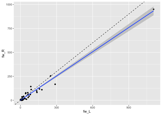
… and across datasets:
da1ds.shared_types.wide %>%
  filter(type!='KCg-m') %>%
  ggplot(data=., aes(fw_R, hb_R)) +
  geom_point() +
  stat_smooth(method = "lm", formula = y ~ x + 0) +
  geom_abline(slope=1, linetype='dashed')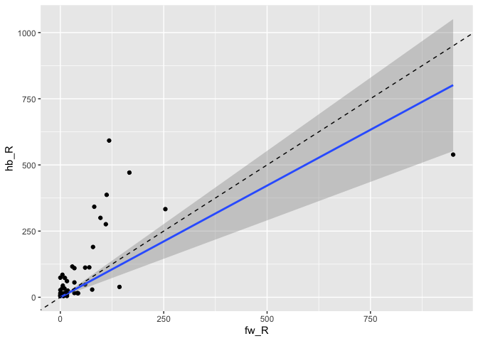
Across dataset connectivity clustering
Being able to fetch shared connectivity in a uniform format is a building block for a range of analyses. For example, we can compare the connectivity of a set of neurons that are believed to constitute the same cell type across multiple datasets. Cosine similarity clustering seems to work very well for this purpose.
cf_cosine_plot(cf_ids('/type:LAL0(08|09|10|42)', datasets = c("flywire", "hemibrain")))
#> Matching types across datasets. Keeping 592/1052 output connections with total weight 15666/24134 (65%)
#> Matching types across datasets. Keeping 694/1493 input connections with total weight 16136/27588 (58%)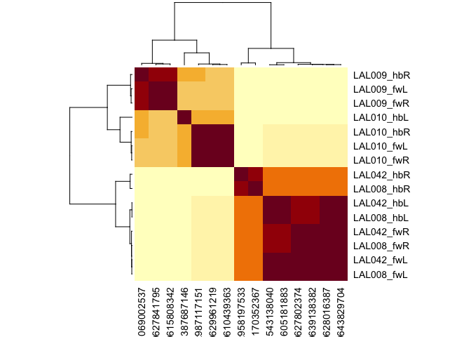
Each row (and column) correspond to a single neuron. Rows are labelled by cell type, dataset and hemisphere; due to truncation hemibrain neurons sometimes exist in one hemisphere, sometimes both. Notice that LAL009 and LAL010 neurons from each hemisphere co-cluster together exactly as we would expect for a cell type conserved across brains. In contrast LAL008 and LAL042 are intermingled; we believe that these constitute a single cell type of two cells / hemisphere (i.e. they should not have been split into two cell types in the hemibrain).
You can also see that cells from one hemibrain hemisphere often cluster slightly oddly (e.g. 387687146) - this is likely due to truncation of the axons or dendrites of these cells or a paucity of partners from the left hand side of the hemibrain.
Going further
We strongly recommend consulting the online manual visible at https://natverse.org/coconatfly/. In particular the vignette(s) listed at https://natverse.org/coconatfly/articles provide full code and instructions for a step by step walk through.
Acknowledgements
Upon publication, please ensure that you appropriately cite all datasets that you use in your analysis. In addition in order to justify continued development of natverse tools in general and coconatfly in particular, we would appreciate two citations for
- For the natverse: Bates et al eLife 2020
- For coconatfly: Schlegel et al Nature 2024
Should you make significant use of natverse packages in your paper (e.g. multiple panels or >1 figure), we would also strongly appreciate a statement like this in the acknowledgements that can be tracked by our funders.
Development of the natverse including the coconatfly and fafbseg packages has been supported by the NIH BRAIN Initiative (grant 1RF1MH120679-01), NSF/MRC Neuronex2 (NSF 2014862/MC_EX_MR/T046279/1) and core funding from the Medical Research Council (MC_U105188491).