“FROM many directions, workers are tunnelling hopefully into the mountain, some with steam shovels and others with dental drills. Some travel blindly in a circle and come out close to their point of entrance; some connect, usually in a mismatched fashion, with the burrows of others. Some have chosen to disregard the random activities of their fellows and have worked out in a small region an elegant system of tunnels of their own. Both the attraction and confusion of this multitudinous excavation lie in the fact that none of these workers knows precisely what they are looking for, or what they will find.” (Kenneth Roeder)
Inspecting the hemibrain
The largest draft connectome to date was released on the 22nd of January, 2020. The FlyEM Janelia HemiBrain project has released 21,662 neurons, many more fragments, and almost 10 million synapses. About 35% of its automatically predicted synapses have been matched up to a semi-automatically traced ‘body’ deemed large enough to constitute an identifiable neuron. This data can be accessed using our R package neuprintr to query a publically accessible neuPrint explorer instance.
Lock and load
# install
if(!require('devtools')) install.packages("devtools")
if(!require('natverse')) devtools::install_github("natverse/natverse")
if (!requireNamespace("BiocManager", quietly = TRUE))install.packages("BiocManager")
if(!require('ComplexHeatmap')) BiocManager::install("ComplexHeatmap")
if(!require('ggnetwork')) install.packages("ggnetwork")
if(!require('network')) install.packages("network")

# load
library(natverse)
library(neuprintr)
library(dendroextras)
library(ComplexHeatmap)
library(ggnetwork)
library(network)

# Colours
## some nice colors!! Inspired by LaCroixColoR
lacroix = c("#C70E7B", "#FC6882", "#007BC3", "#54BCD1", "#EF7C12", "#F4B95A",
            "#009F3F", "#8FDA04", "#AF6125", "#F4E3C7", "#B25D91", "#EFC7E6",
            "#EF7C12", "#F4B95A", "#C23A4B", "#FBBB48", "#EFEF46", "#31D64D",
            "#132157","#EE4244", "#D72000", "#1BB6AF")
names(lacroix) = c("purple", "pink",
                   "blue", "cyan",
                   "darkorange", "paleorange",
                   "darkgreen", "green",
                   "brown", "palebrown",
                   "mauve", "lightpink",
                   "orange", "midorange",
                   "darkred", "darkyellow",
                   "yellow", "palegreen",
                   "navy","cerise",
                   "red", "marine")

## Then see if a simple function works for you:
available.datasets = neuprint_datasets()
available.datasets
If you need help/have not before logged into neuPrint via R, please
see the package README or see ?neuprint_login.
The main point is that you can then edit your R.environ file to
contain information about the neuPrint server you want to speak with,
your token and the dataset hosted by that server, that you want to read.
You can use the package usethis to easily edit your R
environ file. You will need to add these lines to your R environ to
specify the hemibrain dataset:
neuprint_token="YOUR_TOKEN_HERE"
neuprint_server='https://neuprint.janelia.org/'
neuprint_dataset='hemibrain:v1.1'
Leave a blank line at the end of the file.
Then restart your R session.
Find neurons
First, we need to find neurons to read from neuPrint. We can do this easily in two ways - we can search by name, and we can search by brain region.
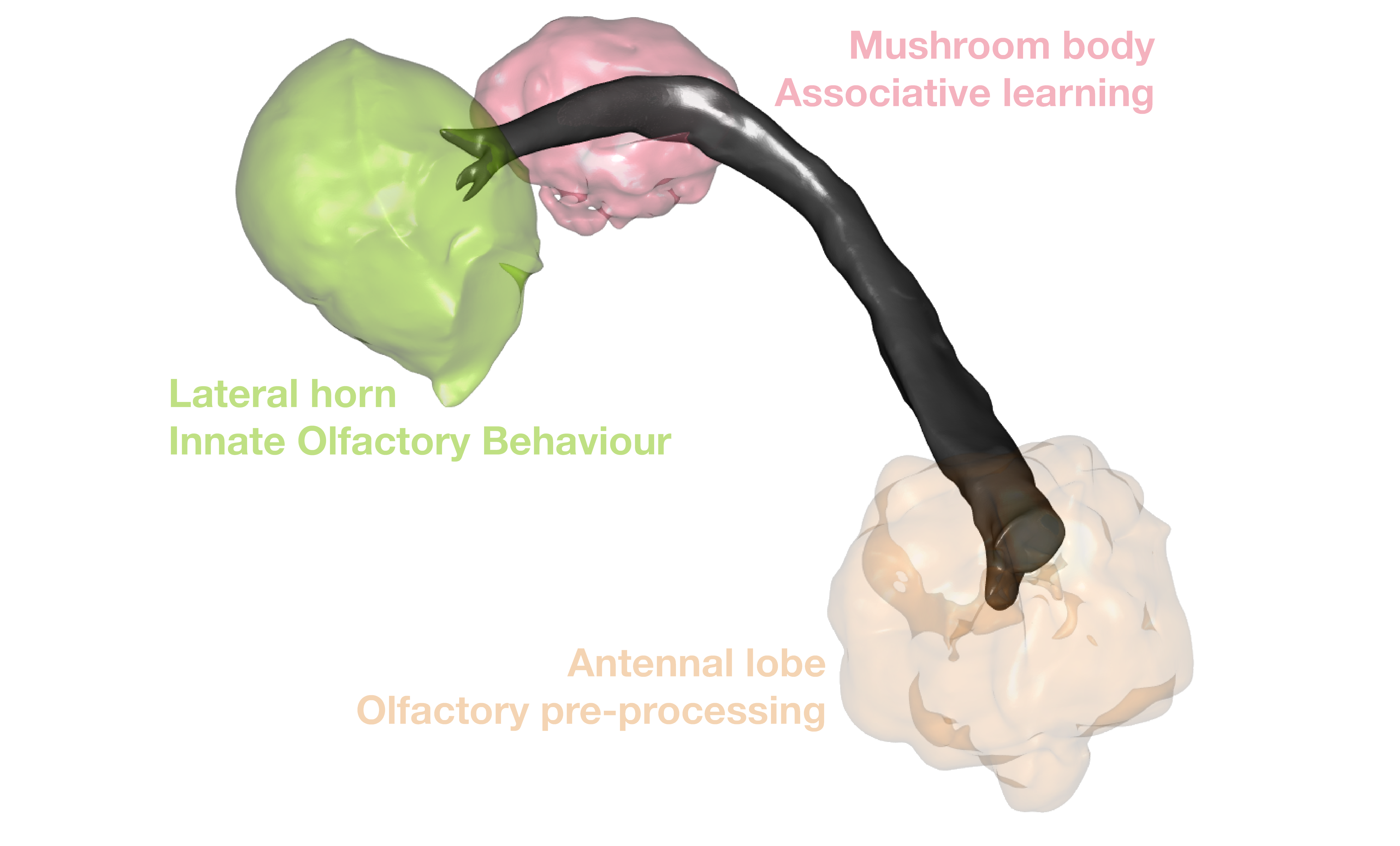
So what do we want to look at? Some of the best studied neurons in the brain are the olfactory projections neurons (OPNs) Grabe et al. 2016. These are second-order olfactory neurons that project from the fly’s equivalent of the olfactory bulb, i.e. the antennal lobe, to higher order brain regions that generate innate behaviours (the lateral horn, LH) (Frechter. 209, Dolan et al. 2019) and learning & memory (the mushroom body) (Aso et al. 2014a, Aso et al. 2014b). We know a fair bit about them, compared with most neurons in the fly brain. For example, a bit of their odour response profiles Badel et al., 2016.
Perhaps we could look at some popular OPN types and see if they connect to each other? How do we get this information?
Let’s find some in our HemiBrain data:
### Let's find some in our HemiBrain data:
opn.info = neuprint_search(".*mPN1.*")
opn.info[is.na(opn.info$type),"type"] = opn.info[is.na(opn.info$type),"name"]
rownames(opn.info) = opn.info$bodyid
#### Add AL glomerulus information from the name
name.split = strsplit(opn.info$name,split=c("\\(|\\_"))
gloms = sapply(name.split, function(x) tryCatch(x[[2]], error = function(e) ""))
names(gloms) = opn.info$bodyid
opn.info$glomerulus = gloms
opn.info = subset(opn.info, glomerulus!="")
#### so there seem to be
print(length(gloms))
#### OPNs and
#### And
print(length(unique(gloms)))
#### OPNs with unique glomerulus innervations
## Let's see what meta-info we get, along with stuff with 'mPN1' in the name.
## This is a reference to the OPN naming scheme by Tanaka et al. (2012)
View(opn.info)
### Looks like we get their unique ID numbers (bodyIds), cell names,
### types, their size (voxels) and synapse numbers (pre=output, post=input).
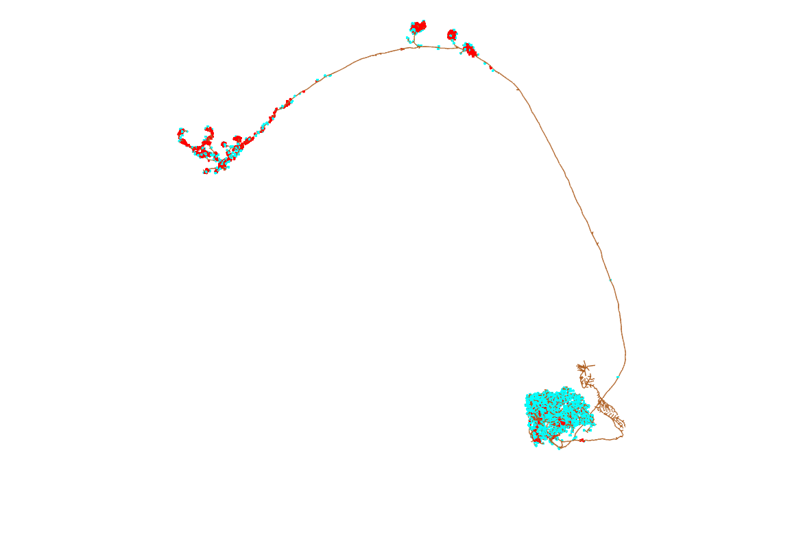
## Let's quickly read one neuron, and have a look at it!
opn = neuprint_read_neuron(opn.info$bodyid[1])
### visualise:
nopen3d(userMatrix = structure(c(0.985064148902893, 0.164582148194313,
0.05061025172472, 0, 0.00997132062911987, -0.347956597805023,
0.93745756149292, 0, 0.171898916363716, -0.922951519489288, -0.344400823116302,
0, 0, 0, 0, 1), .Dim = c(4L, 4L)), zoom = 0.746215641498566,
windowRect = c(20L, 65L, 1191L, 843L)) # set view
plot3d(opn, WithConnectors = TRUE, col = lacroix[["brown"]], lwd = 2)
dir.create("images")
rgl.snapshot(filename = "images/hemibrain_an_opn.png", fmt ="png")
### output synapses in red, input ones in blue
### You can see the auto-segmentation goes a bit crazy where the soma is
## Now that we have all of the bodyIds, we can read these neurons from neuPrint:
opns = neuprint_read_skeletons(opn.info$bodyid)
nopen3d(userMatrix = structure(c(0.98370349407196, -0.104569993913174,
-0.146263062953949, 0, 0.147007316350937, -0.000597098842263222,
0.989135324954987, 0, -0.103521309792995, -0.994517505168915,
0.0147849693894386, 0, 0, 0, 0, 1), .Dim = c(4L, 4L)), zoom = 0.644609212875366,
windowRect = c(20L, 65L, 1191L, 843L))
plot3d(opns, col = sample(lacroix,length(opns), replace = TRUE), lwd = 2)
rgl.snapshot(filename = "images/hemibrain_opns.png", fmt ="png")
## The simple version of read neurons just reads the skeleton for a neuron
### We might also want our neuron objects to contain meta data and synapse information
### We have an all-in-one function to do this. Here we go!
opns = neuprint_read_skeletons(opn.info$bodyid)
##But why is this function so slow?
### Because it fetches fragmented neuron skeletons assigned to the same neuron
### Stitched them into one neuron (healing), grabs all the neuron's synapses
### and tries to work out where the soma is. If you want to move faster
### You can grab bits separately and quickly:
?neuprint_read_skeletons
?neuprint_get_synapses
?neuprint_assign_connectors
?neuprint_locate_soma
?neuprint_get_neuron_names
?neuprint_get_meta
## Do we have to know what's in the name to find interesting neurons? No!
### We can also read neurons from a region of interest (ROI) of the brain.
### The regions of interest available are:
rois = sort(neuprint_ROIs())
rois
## We don't we try fetching all of the neurons in a glomerulus of the mushroom body input zone, the calyx?
ca.info = neuprint_find_neurons(
input_ROIs = "CA(R)",
output_ROIs = NULL,
all_segments = FALSE # if true, fragments smaller than 'neurons' are returned as well
)
## So how many neurons is that?
print(nrow(ca.info))
## A lot! But what about that pesky load of Kenyon cells
### The most populous neurons in the brain
ca.info = subset(ca.info, !is.na(bodyname) & neuronStatus == "Traced")
ca.info = ca.info[!grepl("KC",ca.info$bodyname),]
## So how many neurons is that?
print(nrow(ca.info))
## Getting all that data took a while, so let's save it for later
save(opns,file = "hemibrain_opns.rda")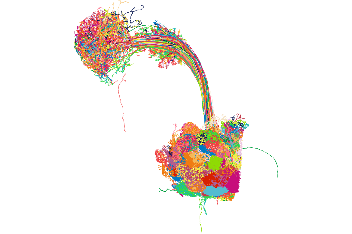
Get neuropil volumes
So it is nice that we now have some neurons. But it would be good to see them with their neuropil context.
Let’s fetch some volume data to plot:
## Let's get some neuropil volume data from neuPrint!
### Specifically, in the last R file we chose to look at OPNs
### So let's fetch their meshes for the antennal lobe!
### First, we gotta see what is available:
rois
# Read in the AL mesh!
al.mesh = neuprint_ROI_mesh(roi = "AL(R)")
nopen3d(userMatrix = structure(c(0.947127282619476, 0.222770735621452,
-0.230919197201729, 0, 0.247805655002594, -0.0506941750645638,
0.967482566833496, 0, 0.203820571303368, -0.973551869392395,
-0.103217624127865, 0, 0, 0, 0, 1), .Dim = c(4L, 4L)), zoom = 0.58467960357666,
windowRect = c(1460L, 65L, 2877L, 996L)) # set view
plot3d(al.mesh, add = TRUE, alpha = 0.1, col = lacroix[["orange"]])
# And get the other main olfactory neuropils
ca.mesh = neuprint_ROI_mesh(roi = "CA(R)")
lh.mesh = neuprint_ROI_mesh(roi = "LH(R)")
malt.mesh = neuprint_ROI_mesh(roi = "mALT(R)")
plot3d(ca.mesh, add = TRUE, alpha = 0.3, col = lacroix[["pink"]])
plot3d(lh.mesh, add = TRUE, alpha = 0.3, col = lacroix[["green"]])
plot3d(malt.mesh, add = TRUE, alpha = 0.9, col = "grey30")
rgl.snapshot(filename = "images/hemibrain_olfactory_neuropils.png", fmt ="png")
## Maybe get the whole hemibrai mesh?
## hemibrain = neuprint_ROI_mesh(roi = "hemibrain")
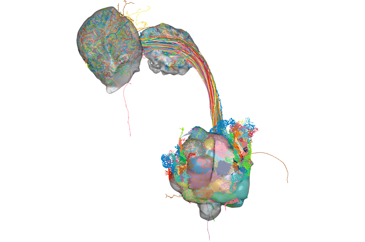
# And with some neurons!
nopen3d(userMatrix = structure(c(0.98370349407196, -0.104569993913174,
-0.146263062953949, 0, 0.147007316350937, -0.000597098842263222,
0.989135324954987, 0, -0.103521309792995, -0.994517505168915,
0.0147849693894386, 0, 0, 0, 0, 1), .Dim = c(4L, 4L)), zoom = 0.644609212875366,
windowRect = c(20L, 65L, 1191L, 843L))
plot3d(al.mesh, add = TRUE, alpha = 0.5, col = "grey")
plot3d(ca.mesh, add = TRUE, alpha = 0.5, col = "grey")
plot3d(lh.mesh, add = TRUE, alpha = 0.5, col = "grey")
plot3d(opns, col = sample(lacroix,length(opns), replace = TRUE), lwd = 2)
rgl.snapshot(filename = "images/hemibrain_opns_neuropils.png", fmt ="png")Here is what the neurons look like with these brain meshes:
Get connectivity
And now the really exciting bit! How do these neurons connect to each other?
First we will look at connectivity between OPN types.
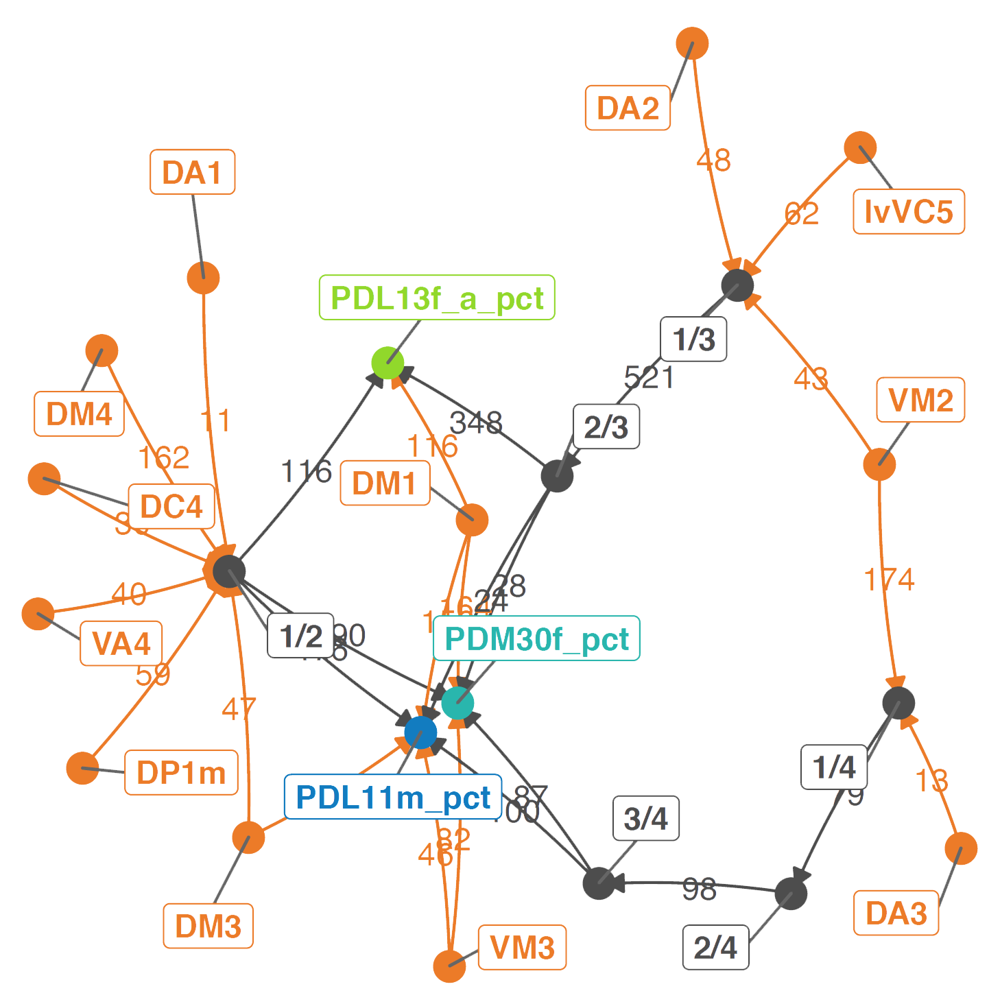
Then we will follow up on their connectivity with other neurons in the brain. We will focus on the uniglomerular projection neuron (uPN) from the apple cider vinegar detecting glomerulus, DM1. It is already known that it is a hub for connectivity in the lateral horn, impinging on the axons of other food-odour related projection neurons (Bates and Schlegel et al., 2020). We’ll see in the code below, that we can find that this PNs’ (orange) strongest downstream targets include these neurons in the lateral horn (the part of the brain that generates ‘innate’ behaviours):
And that other uPNs can influence them both directly and via interstitial neurons:
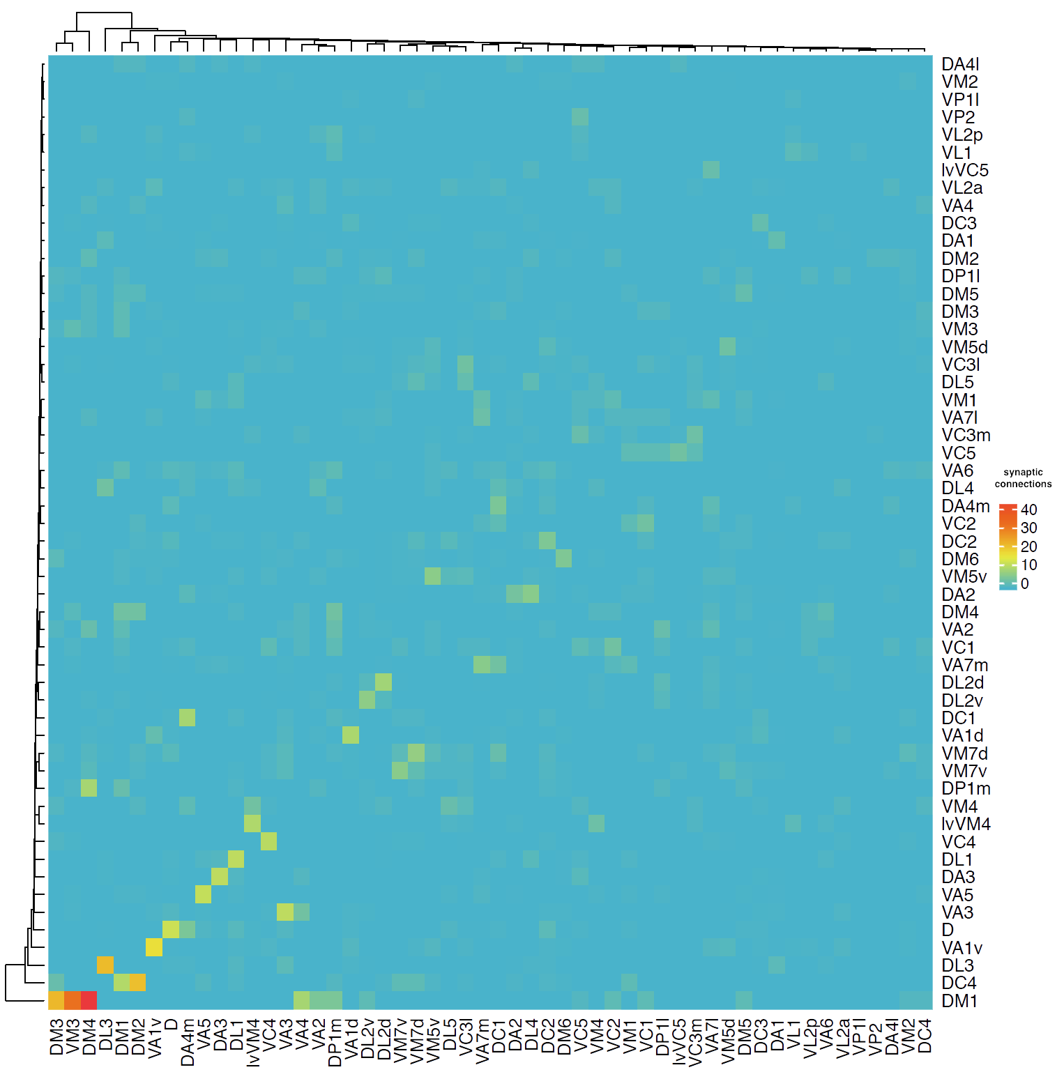
## We are looking at connectivity between OPNs.
### We can get an adjaceny matrix between all of these OPNs
opn.adj = neuprint_get_adjacency_matrix(bodyids = opn.info$bodyid)
rownames(opn.adj) = colnames(opn.adj) = opn.info$type
## Let's visualise this connectivity
my_palette <- colorRampPalette(c(lacroix[["cyan"]],lacroix[["yellow"]], lacroix[["orange"]], lacroix[["cerise"]])) (n=20)
pdf(file = "images/OPN_interconnectivity.pdf", height = 10, width = 10)
Heatmap(opn.adj,
col = my_palette)
dev.off()
## It is hard to parse this information mentally
### What if we just see what the glomerulus to glomerulus connectivity is?
opn.adj.comp = opn.adj
rownames(opn.adj.comp) = colnames(opn.adj.comp) = opn.info$glomerulus
opn.adj.comp = t(apply(t(opn.adj.comp), 2, function(x) tapply(x, colnames(opn.adj.comp), sum, na.rm = TRUE)))
opn.adj.comp = apply(opn.adj.comp, 2, function(x) tapply(x, rownames(opn.adj.comp), sum, na.rm = TRUE))
pdf(file = "images/OPN_glomerulus_interconnectivity.pdf", height = 10, width = 10)
Heatmap(opn.adj.comp,
col = my_palette)
dev.off()
## What about OPN connectivity to neurons not in this set of OPNs?
### First, is there a common partner to all OPNs?
common = neuprint_common_connectivity(opn.info$bodyid, prepost = "PRE") # could use 'post' for downstream
dim(common)
### What about the food hub PNs?
### The glomerulus DM1 is interesting, because it is involved in an axo-axonic
### 'food odour' related community in the lateral horn (Bates & Schlegel et al. 2020)
DM1.opn.info = subset(opn.info, grepl("DM1|DM3|DM4|VM3|VA4",name))
DM1.common = neuprint_common_connectivity(DM1.opn.info$bodyid, prepost = "PRE")
dim(DM1.common)
DM1.common.meta = neuprint_get_meta(colnames(DM1.common)) # what are they?
View(DM1.common.meta) # Huhh, local neurons, the APL and some LH stuff
## Another interesting question we can ask is whether PNs get axonic inouts in the calyx
### from Kenyon cells (KCs). In their other axon collateral in the LH it has already been shown
### That they get innervation from local neurons.
kc.info = neuprint_search("KC.*")
opn.conn = neuprint_connection_table(bodyids = opn.info$bodyid, prepost = "PRE")
opn.conn = opn.conn[opn.conn$partner%in%kc.info$bodyid,]
opn.conn$glom = gloms[as.character(opn.conn$bodyid)]
glom.conn = aggregate(list(weight = opn.conn$weight),
list(glom = opn.conn$glom,
prepost = opn.conn$prepost),
sum)
table(opn.conn$weight) # Most barely connect
hist(opn.conn$weight, breaks = 9)
hist(glom.conn$weight, breaks = max(glom.conn$weight)/10) # However if you add up by uPN cell type, the numbers can look high
## We can also get all of the neurons in the database that connect to the
### query neurons, either upstream or downstream of them
DM1.opn.connected = neuprint_connection_table(DM1.opn.info$bodyid, prepost = "POST")
### In which brain region are these partners?
table(DM1.opn.connected$roi)
## Important note!!
### The results from neuprint_connection_table can list the same bodyid-partner pairing
### multiple times if by.roi = TRUE. This is because there is a separate entry for each of FlyEM's designated
### regions of interest (ROIs), and because a super-level ROI can include multiple smaller ROIs.
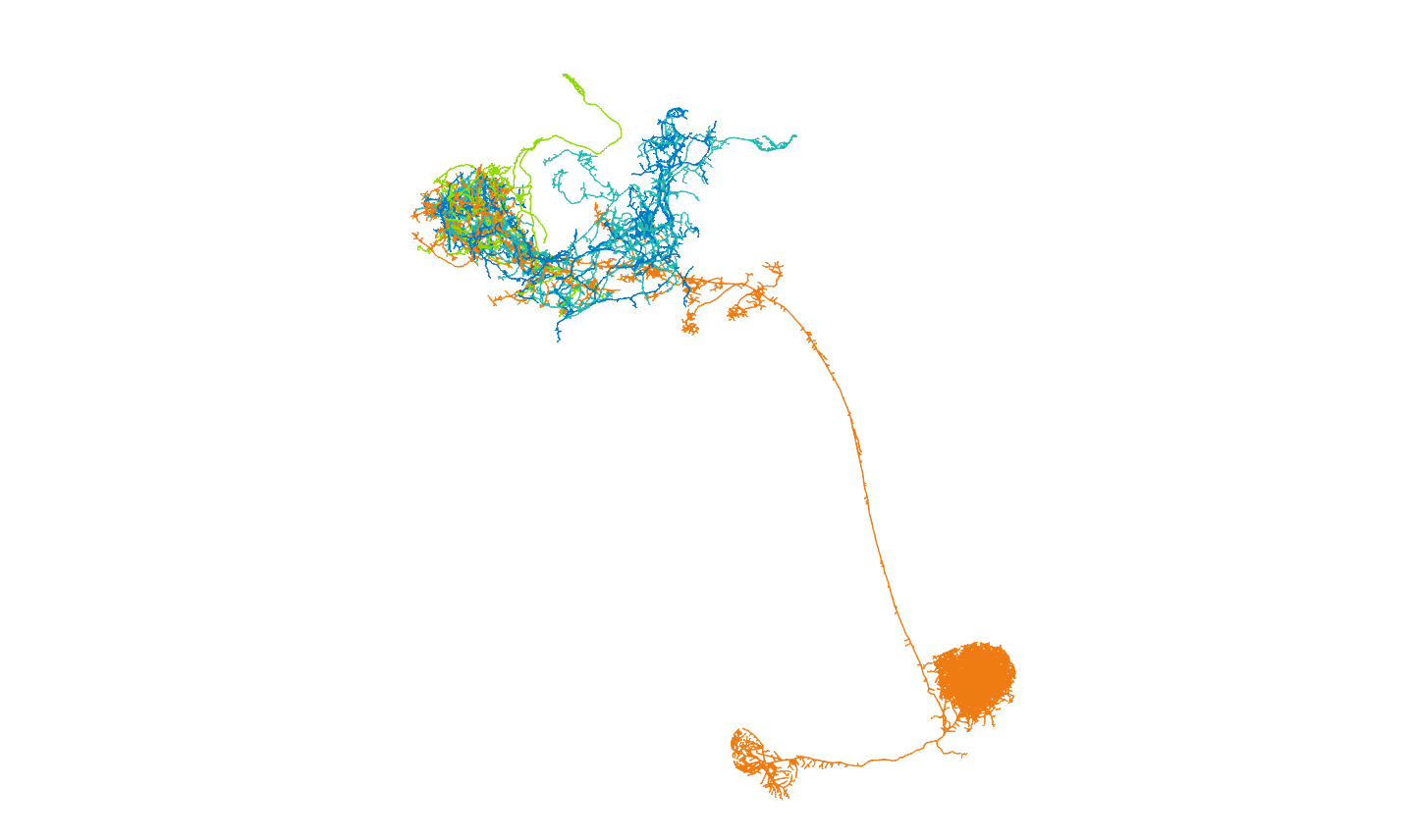
## Let's have a look at what the strongest downstream partners look like
DM1.opn.connected.strong = subset(DM1.opn.connected,weight>100, prepost = "POST")
DM1.targets = neuprint_read_neurons(DM1.opn.connected.strong$partner)
DM1.targets = unspike(DM1.targets, threshold=1000)
nopen3d(userMatrix = structure(c(0.964227318763733, -0.0444099828600883,
-0.261329621076584, 0, 0.249727189540863, -0.178416073322296,
0.951737523078918, 0, -0.088891975581646, -0.982952415943146,
-0.160943150520325, 0, 0, 0, 0, 1), .Dim = c(4L, 4L)), zoom = 0.783526360988617,
windowRect = c(-6L, 71L, 1434L, 927L))
plot3d(DM1.targets, lwd = 2, col = sample(lacroix,length(DM1.targets),replace=TRUE))
rgl.snapshot(filename = "images/hemibrain_DM1_strong_downstream_partners.png", fmt ="png")
View(DM1.targets[,])
## So there are three lateral horn neuron targets of the axon there
### c("359214479", "359891881", "511616870"), found using nat::find.neuron
### Let's move forward with those
lhns = c("359214479", "359891881", "511616870")
lhn.cols = c(lacroix[["marine"]],lacroix[["blue"]],lacroix[["green"]])
names(lhn.cols) = DM1.targets[lhns,"type"]
lh.targets = DM1.targets[lhns]
clear3d()
plot3d(lh.targets, lwd = 2, col = c(lacroix[["marine"]],
lacroix[["blue"]],
lacroix[["green"]]))
plot3d(subset(opns,grepl("DM1",name)),lwd=2,col=lacroix[["orange"]])
rgl.snapshot(filename = "images/hemibrain_DM1_strong_LH_targets.png", fmt ="png")
## Can other OPNs influence these strong partners?
### Which other OPNs impinge on it?
### Via whatever path?
shortest.paths = data.frame()
for(lhn in lhns){
for(b in opn.info$bodyid){ # PN -> LHN
sp = neuprint_get_shortest_paths(body_pre = b, body_post = lhn, weightT = 10)
dupe = ifelse( is.na(which(duplicated(sp$to))[1]),nrow(sp),which(duplicated(sp$to))[1])
shortest = sp[1:dupe,]
if(nrow(shortest)>0 & nrow(shortest)<5 ){
shortest$order.to = paste(1:nrow(shortest), nrow(shortest), sep = "/")
shortest$order.from = paste(1:nrow(shortest)-1, nrow(shortest), sep = "/")
shortest[1,"order.from"] = opn.info[as.character(b),"glomerulus"]
shortest[nrow(shortest),"order.to"] = DM1.targets[lhn,"type"]
shortest.paths = rbind(shortest.paths, shortest)
}
}
for(b in opn.info$bodyid){ # LHN -> PN
sp = neuprint_get_shortest_paths(body_post = b, body_pre = lhn, weightT = 5)
dupe = ifelse( is.na(which(duplicated(sp$to))[1]),nrow(sp),which(duplicated(sp$to))[1])
shortest = sp[1:dupe,]
if(nrow(shortest)>0 & nrow(shortest)<2){
shortest[1,"order.from"] = opn.info[as.character(b),"glomerulus"]
shortest[nrow(shortest),"order.to"] = DM1.targets[lhn,"type"]
shortest.paths = rbind(shortest.paths, shortest)
}
}
}
# Make network
set.seed(42)
paths = aggregate(list(weight = shortest.paths$weight), list(order.from = shortest.paths$order.from,
order.to = shortest.paths$order.to),
sum)
n = network(paths,
matrix.type = "edgelist",
ignore.eval = FALSE,
layout = "fruchtermanreingold",
names.eval = "weight",
directed = TRUE)
n = ggnetwork(n, cell.jitter = 0.75, arrow.gap = 0.01)
# Set colours
orders = unique(c(paths$order.to,paths$order.from))
order.cols = rep("grey30",length(orders))
names(order.cols) = orders
gloms = unique(opn.info$glomerulus)
opn.cols = rep(lacroix[["orange"]],length(gloms))
names(opn.cols) = gloms
opn.cols = c(opn.cols,lhn.cols,order.cols[!names(order.cols)%in%c(names(lhn.cols),names(opn.cols))])
# Plot
set.seed(1)
pdf(file = "images/DM1_OPN_input_graph.pdf", height = 5, width = 5)
ggplot(n, aes(x = x, y = y, xend = xend, yend = yend)) +
geom_edges(aes(color = vertex.names),
curvature = 0.05,
arrow = arrow(length = unit(6, "pt"),
type = "closed")) +
geom_nodes(aes(color = vertex.names, size = 6)) +
geom_edgetext(aes(label = weight, color = vertex.names), fill = NA) +
geom_nodelabel_repel(aes(color = vertex.names, label = vertex.names),
fontface = "bold", box.padding = unit(1, "lines")) +
scale_color_manual(values = opn.cols) +
scale_fill_manual(values = opn.cols) +
theme_blank() +
guides(color = FALSE, shape = FALSE, fill = FALSE, size = FALSE, linetype = FALSE) + ylab("") + xlab("")
dev.off()Article
A Connectome of the Adult Drosophila Central Brain
Shan Xu, C; Januszewski, Michal; Lu, Zhiyuan; Takemura, Shin-Ya; Hayworth, Kenneth; Huang, Gary; Shinomiya, Kazunori; Maitin-Shepard, Jeremy; Ackerman, David; Berg, Stuart; Blakely, Tim; Bogovic, John; Clements, Jody; Dolafi, Tom; Hubbard, Philip; Kainmueller, Dagmar; Katz, William; Kawase, Takashi; Khairy, Khaled; Leavitt, Laramie; Li, Peter H; Lindsey, Larry; Neubarth, Nicole; Olbris, Donald J; Otsuna, Hideo; Troutman, Eric T; Umayam, Lowell; Zhao, Ting; Ito, Masayoshi; Goldammer, Jens; Wolff, Tanya; Svirskas, Robert; Schlegel, Philipp; Neace, Erika R; Knecht, Christopher J; Alvarado, Chelsea X; Bailey, Dennis; Ballinger, Samantha; Borycz, Jolanta A; Canino, Brandon; Cheatham, Natasha; Cook, Michael; Dreyer, Marisa; Duclos, Octave; Eubanks, Bryon; Fairbanks, Kelli; Finley, Samantha; Forknall, Nora; Francis, Audrey; Hopkins, Gary Patrick; Joyce, Emily M; Kim, Sungjin; Kirk, Nicole A; Kovalyak, Julie; Lauchie, Shirley A; Lohff, Alanna; Maldonado, Charli; Manley, Emily A; McLin, Sari; Mooney, Caroline; Ndama, Miatta; Ogundeyi, Omotara; Okeoma, Nneoma; Ordish, Christopher; Padilla, Nicholas; Patrick, Christopher; Paterson, Tyler; Phillips, Elliott E; Phillips, Emily M; Rampally, Neha; Ribeiro, Caitlin; Robertson, Madelaine K; Rymer, Jon Thomson; Ryan, Sean M; Sammons, Megan; Scott, Anne K; Scott, Ashley L; Shinomiya, Aya; Smith, Claire; Smith, Kelsey; Smith, Natalie L; Sobeski, Margaret A; Suleiman, Alia; Swift, Jackie; Takemura, Satoko; Talebi, Iris; Tarnogorska, Dorota; Tenshaw, Emily; Tokhi, Temour; Walsh, John J; Yang, Tansy; Horne, Jane Anne; Li, Feng; Parekh, Ruchi; Rivlin, Patricia K; Jayaraman, Vivek; Ito, Kei; Saalfeld, Stephan; George, Reed; Meinertzhagen, Ian; Rubin, Gerald M; Hess, Harald F; Scheffer, Louis K; Jain, Viren; Plaza, Stephen M
bioRxiv, Jan 21, 2020 10.1101/2020.01.21.911859